Structure Determination

Where do these structures come from anyway?

8/31/2026

print view

Many images/slides courtesy Andrew VanDemark and https://www.xtal.iqfr.csic.es/Cristalografia/

%%html
<script src="https://bits.csb.pitt.edu/preamble.js"></script>

%%html
<div id="bigmut1" style="width: 500px"></div>
<script>
    var divid = '#bigmut1';
	jQuery(divid).asker({
	    id: divid,
	    question: "Which mutation do you think would be most likely to effect protein function?",
		answers: ["L->V","K->R","A->W","N->Q"],
        server: "https://bits.csb.pitt.edu/asker.js/example/asker.cgi",
		charter: chartmaker})
    
$(".jp-InputArea .o:contains(html)").closest('.jp-InputArea').hide();


</script>

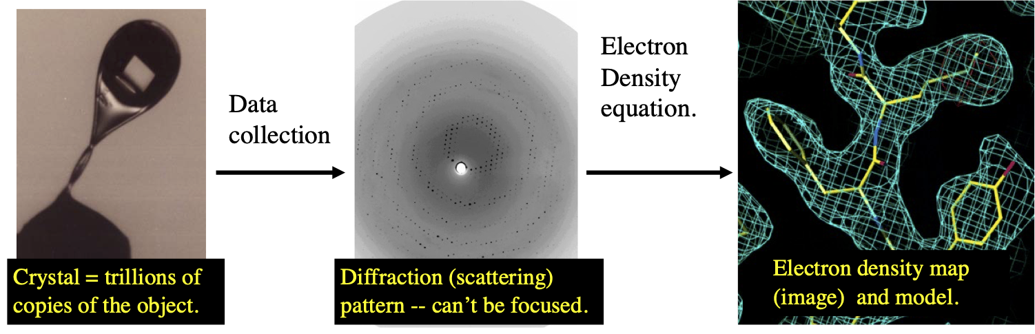
How can we "see" the atoms of a protein?

PDB Structures

2022 2025 2026

Total: 194,820 241,345 259,129

X-Ray Crystallography: 168,396 (86.4%) 197,195 (81.7%) 206,950 (79.9%)

NMR: 13,781 (7.1%) 14,578 (6.0%) 14,828 (5.7%)

Electron Microscopy: 12,323 (6.3%) 28,822 (11.9%) 36564 (14.1%)

X-Ray Crystallography

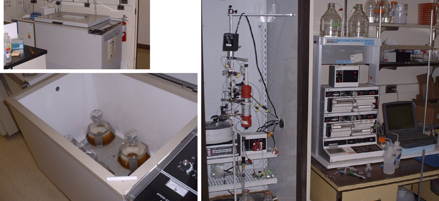
Step 0: Protein Purification

Crystallographic studies usually start with at least 10mg of highly pure protein (huge amount).

Proteins are usually expressed recombinantly in E.coli.

Step 1: Get Your Crystal

Vapor Diffusion

A droplet, either hanging (A) or sitting (B), with protein and low concentrations of precipitant (e.g. salt) gradually equalizes with a resevior with high concentrations of precipitant.

Microdialysis

A semi-permeable membrane is used instead of an "air gap".

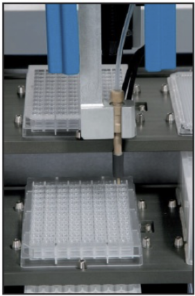
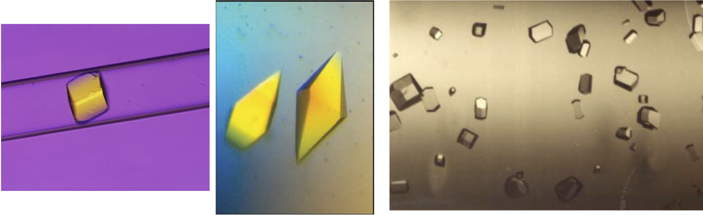
Get Your Crystal

Success of crystallization is sensitive to a number of factors (temperature, pH, buffer contents). The right conditions are found through automated search with robots.

Good Crystals

Crystals are a Lattice of Proteins

Electron Micrograph of Rhombohedral Canavalin

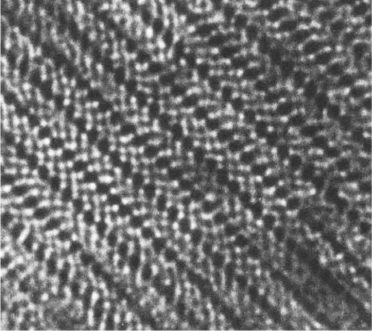
Crystal Terms:

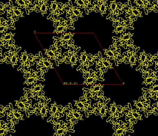
Unit Cell

The repeating unit of the lattice.

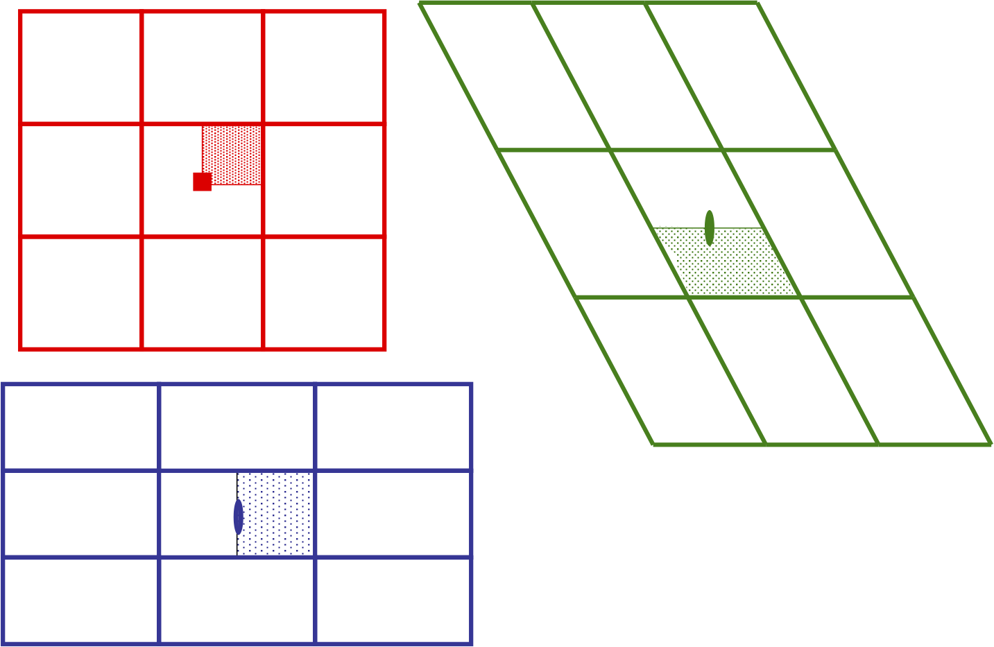
Asymmetric Unit

The smallest volume for which the unit cell can be reconstructed by applying symmetry operations.

Space Group

The set of geometrical symmetry operations that take a three-dimensional periodic object (i.e. the crystal) into itself. The total number of crystallographic space groups is 230.

Examples

v = py3Dmol.view(query='url:https://3dmol.org/tests/test_structs/multi.cif',style='stick',options={'doAssembly':True,'duplicateAssemblyAtoms':True,'normalizeAssembly':True}); v.addUnitCell(); v.show()       

3Dmol.js failed to load for some reason. Please check your browser console for error messages.

Step 2: X-Ray Your Crystal

Go to your neighborhood synchrotron...

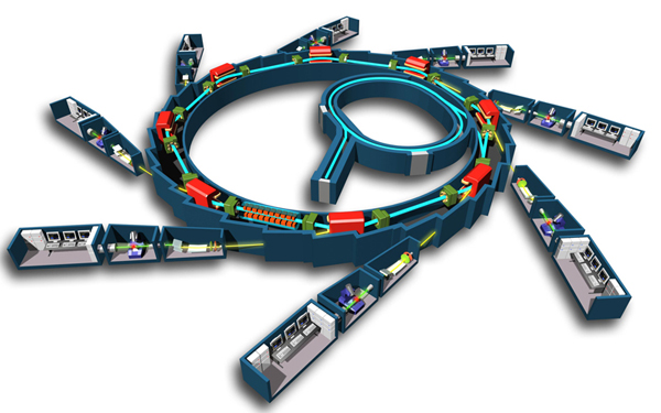
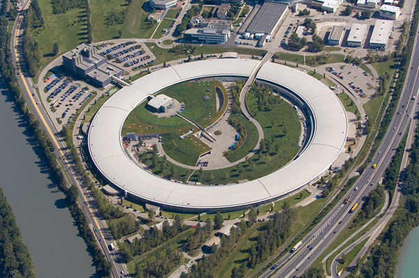
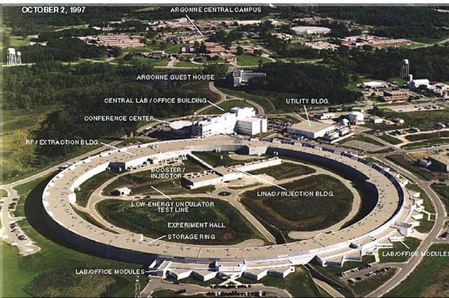
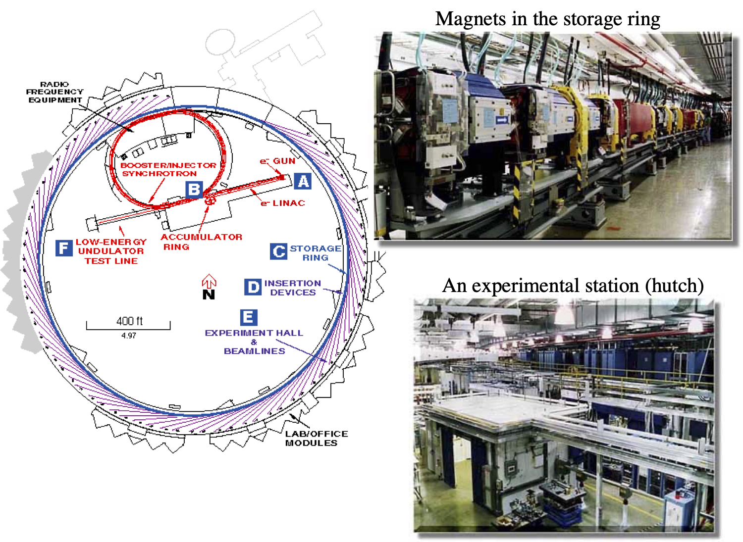
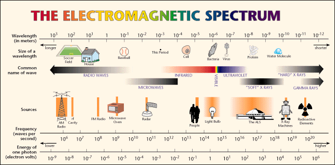
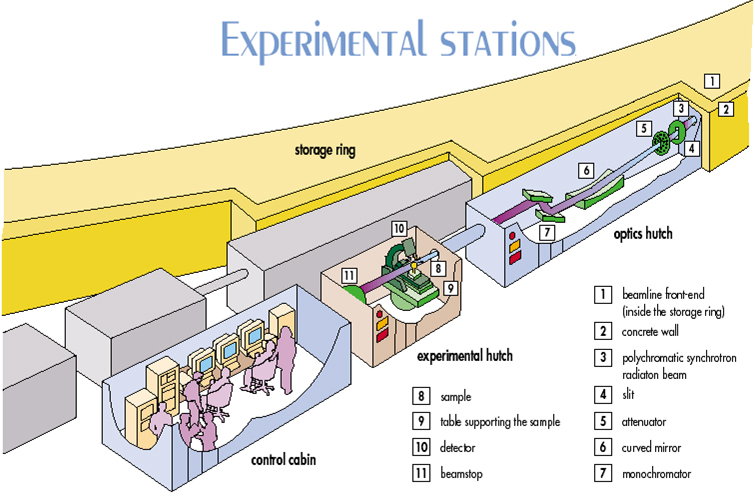
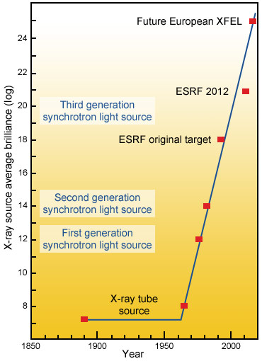
Why Synchrotrons?

Diffraction

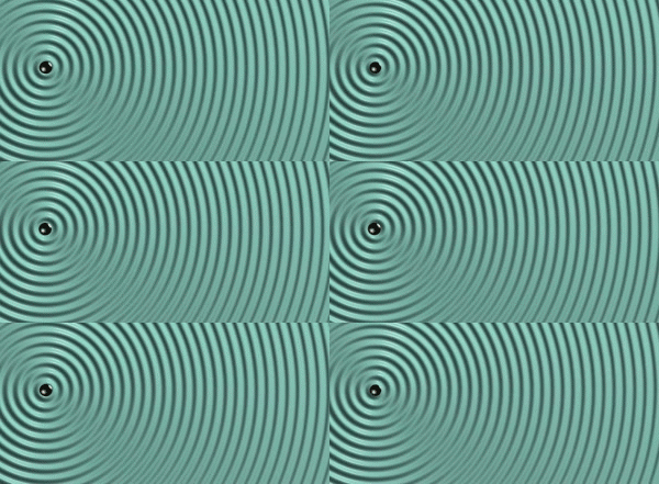
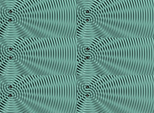
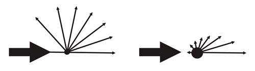
Single electron scattering vs. atom scattering (multiple electrons).

^{Animations originally taken from physics-animations.com}

Experimental Diffraction

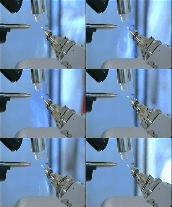
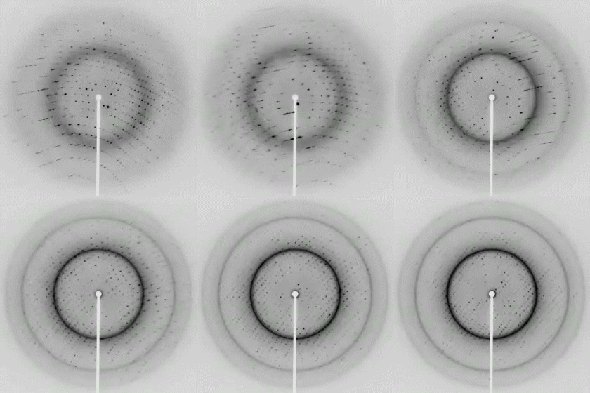
Crystal is mounted on a goniometer (fancy name for something that rotates the crystal).

Cold (-170C) nitrogen cools the crystal.

Crystal Diffraction

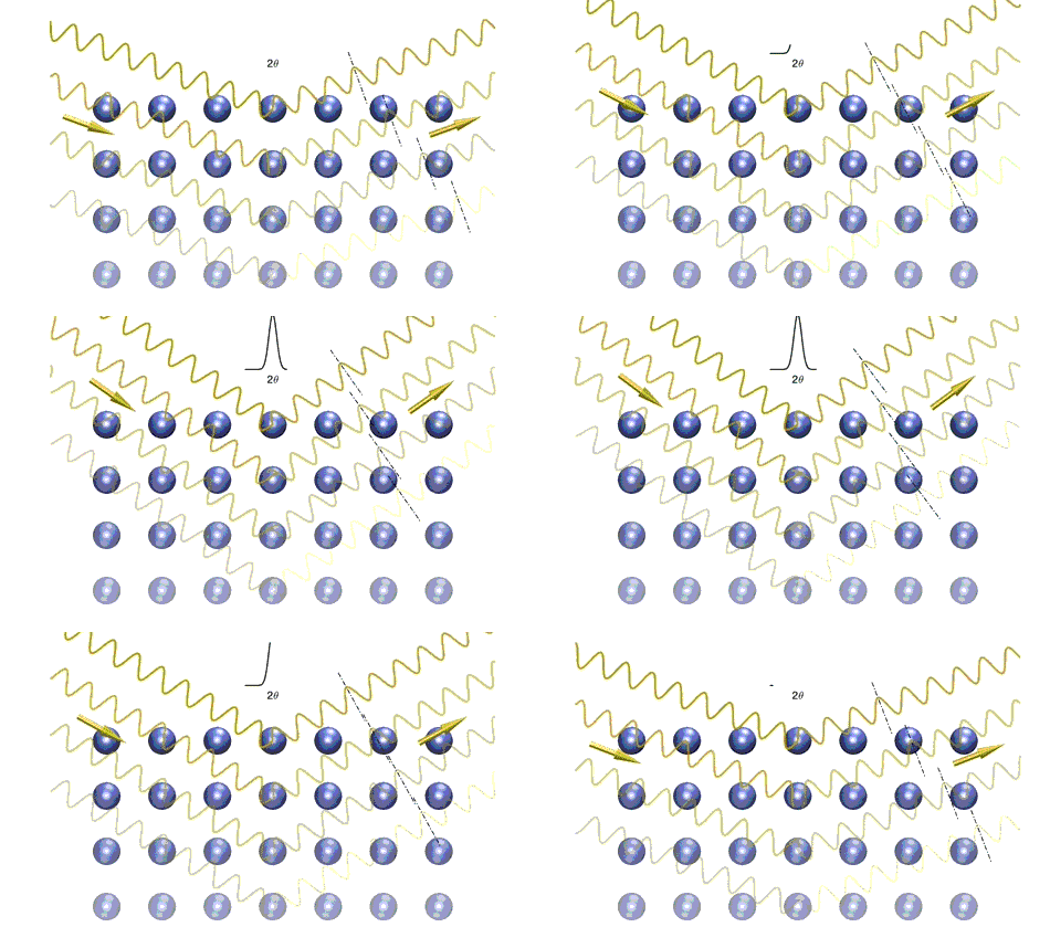
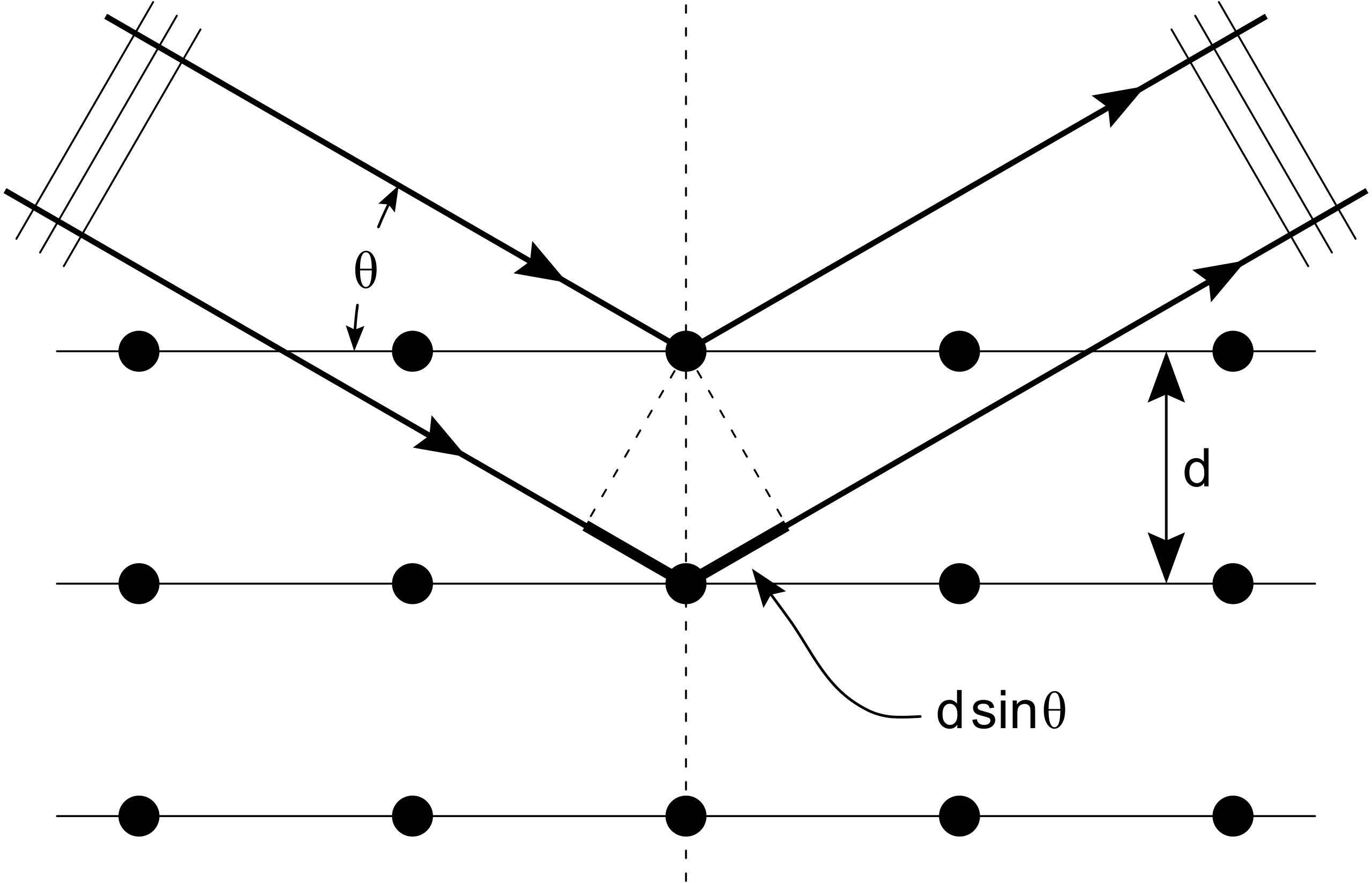
In a lattice, only some angles will result in an output signal due to interference.

Bragg's Law

$$\huge n\lambda = 2 d\sin\theta$$

By Hydrargyrum - Own work, CC BY-SA 3.0, Link

Atomic Scattering Factors

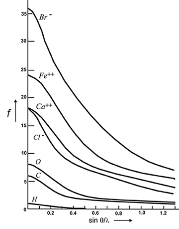
An atomic scattering factor (amplitude), $f$, can be computed (from QM) for every atom. It is a function of the scattering angle, $\theta$ and the X-ray wavelength, $\lambda$.

Thermal (B) Factors

Due to thermal vibrations within the material, the effective volume of the atom appears larger, leading to an exponential decrease of the scattering power, characterized by a coefficient B

$$H = 2 \frac{\sin \theta}{\lambda}$$ $$ f_{\mathrm{thermal}} = f(H) e^{-B \frac{\sin^2\theta}{\lambda^2}}$$

In theory $B$ is the quadratic average amplitude of thermal vibration and can be computed.

In practice it ends up being a bit of a fudge factor.

Crystal Diffraction

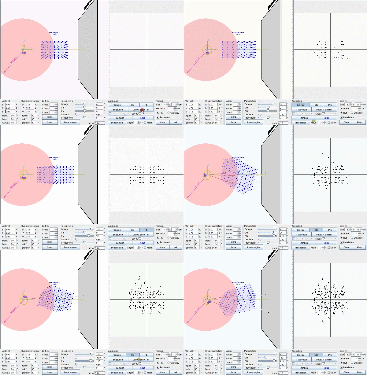
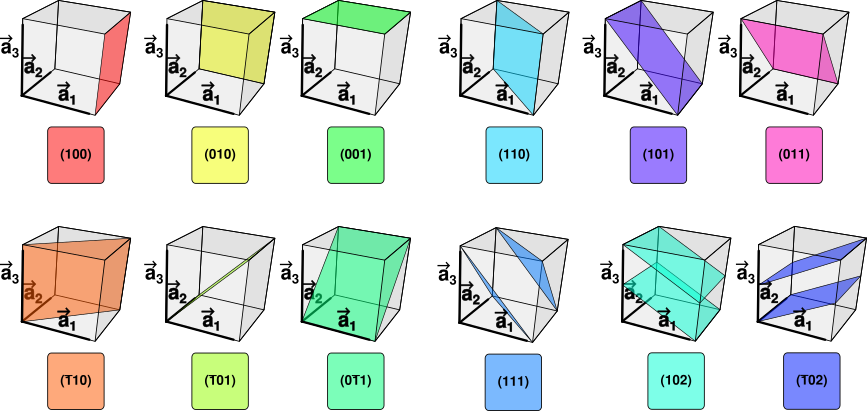
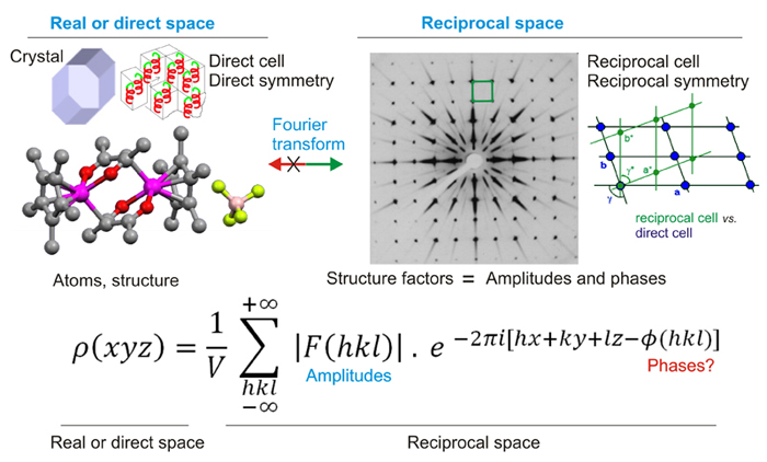
These output signals define positions in a reciprocal lattice with positions $h,k,l$.

Miller Indices

Basis vectors of reciprocal lattice.

%%html
<div id="whatcoole" style="width: 500px"></div>
<script>
    var divid = '#whatcoole';
	jQuery(divid).asker({
	    id: divid,
	    question: "What will be most effected by temperature?",
		answers: ["h","k","l","B"],
        server: "https://bits.csb.pitt.edu/asker.js/example/asker.cgi",
		charter: chartmaker})
    
$(".jp-InputArea .o:contains(html)").closest('.jp-InputArea').hide();


</script>

Resolution of Reflections

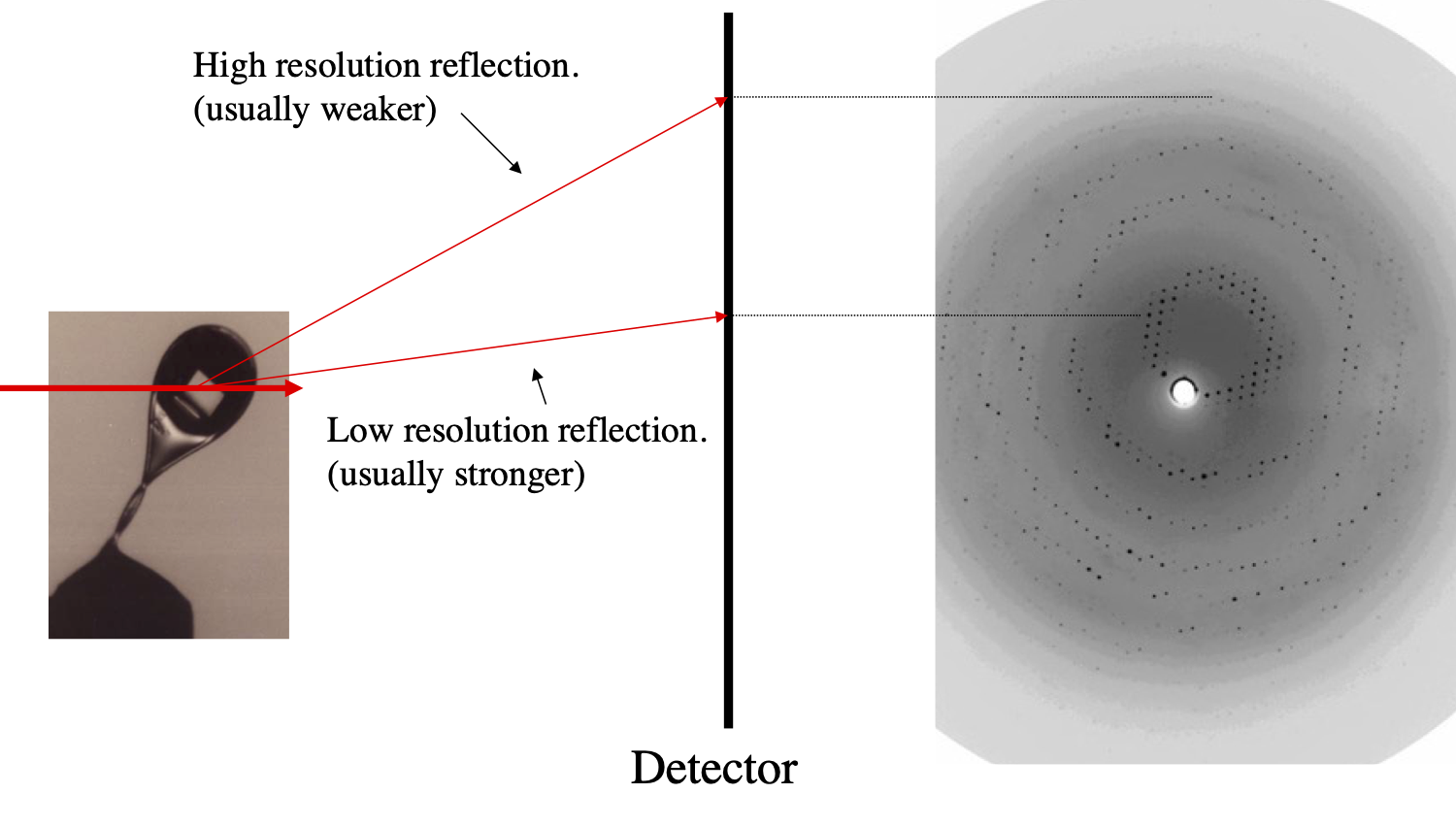
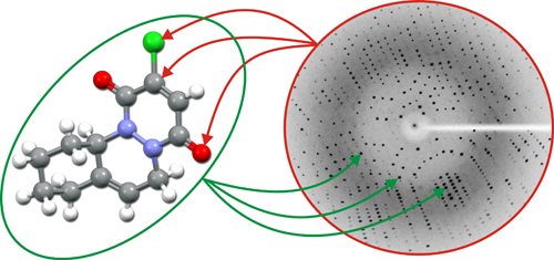
Each "dot" in the diffraction patter is called a reflection.

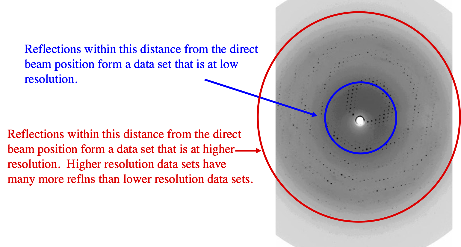
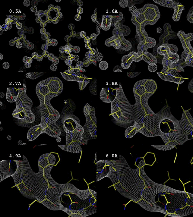
The higher the scattering angle the higher the resolution and the more detail that can be visualized.

Overall Resolution

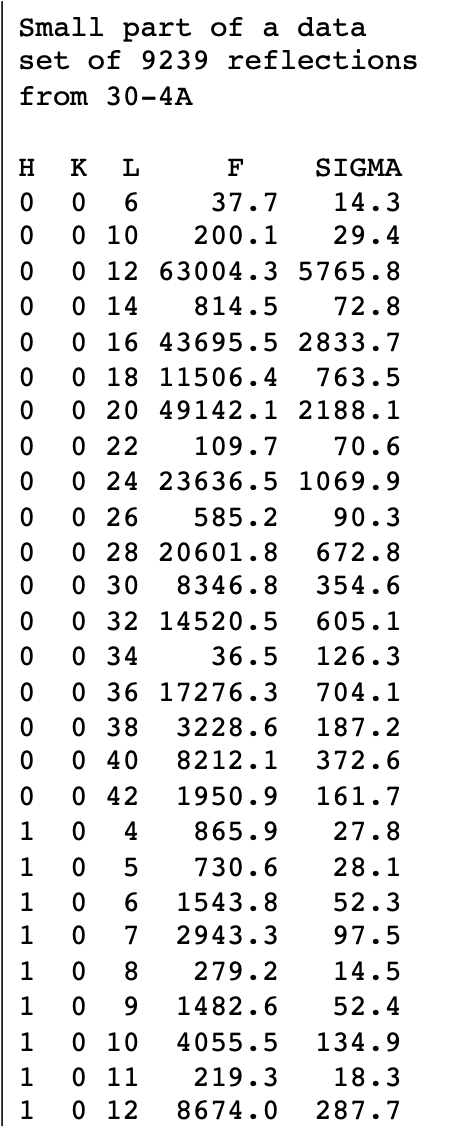
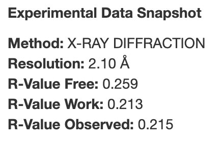
"The resolution of the data set is defined as the resolution at which the intensity of half of the reflections falls to less than 2 times their standard deviation."

Resolution is specified in Angstroms and indicates the ability resolve features that are closer than a given distance.

Resolution Key Points

Average measure of the quality of the diffraction data source

High resolution has a small number.

Resolution

5.0A	3.0A	1.7A

Generally want < 3.0A.

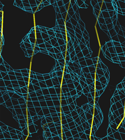
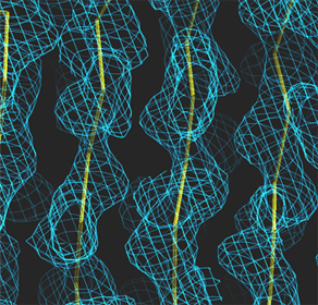
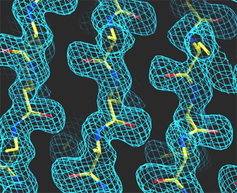
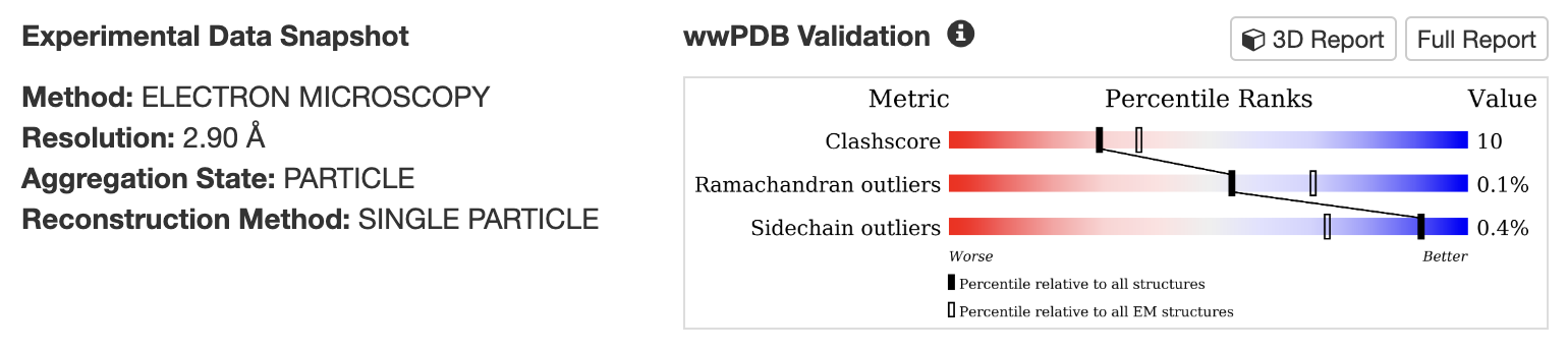
Resolution

Step 3: Determine Electron Density from Diffraction Pattern

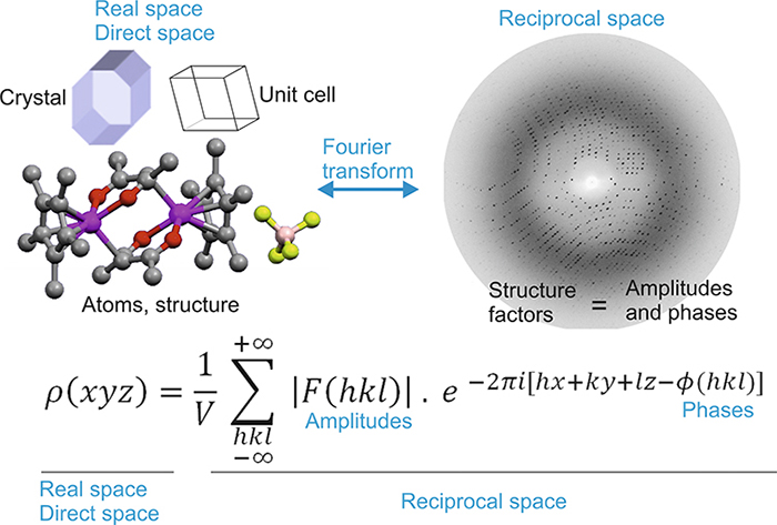
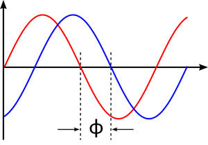
The electron density at position $xyz$ ($\rho(xyz)$) of a unit cell with volume $V$ is related to the diffraction pattern, which has peaks of amplitude $F(hkl)$ at positions $hkl$ through a Fourier transform.

What is the (Discrete) Fourier Transform?

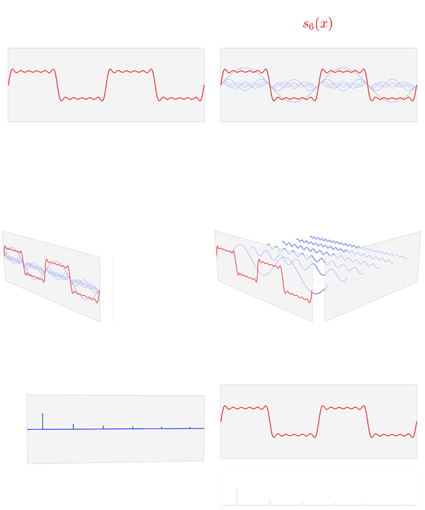
A transformation from "real" space to frequency space. Represent (almost) any function sampled at $N$ uniformly spaced points with $N$ periodic functions (frequency domain).

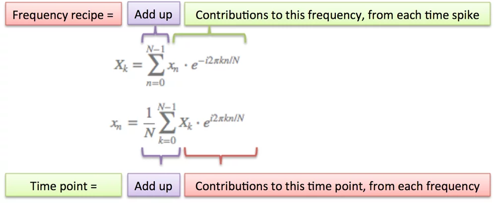
$$\Large X_k = \sum_{n=0}^{N-1} x_n \cdot e^{-\frac {i 2\pi}{N}kn}$$

$x_n = $ value of some function at the $n$th point

$k = $ the $k$th frequency

$i = \sqrt{-1}$

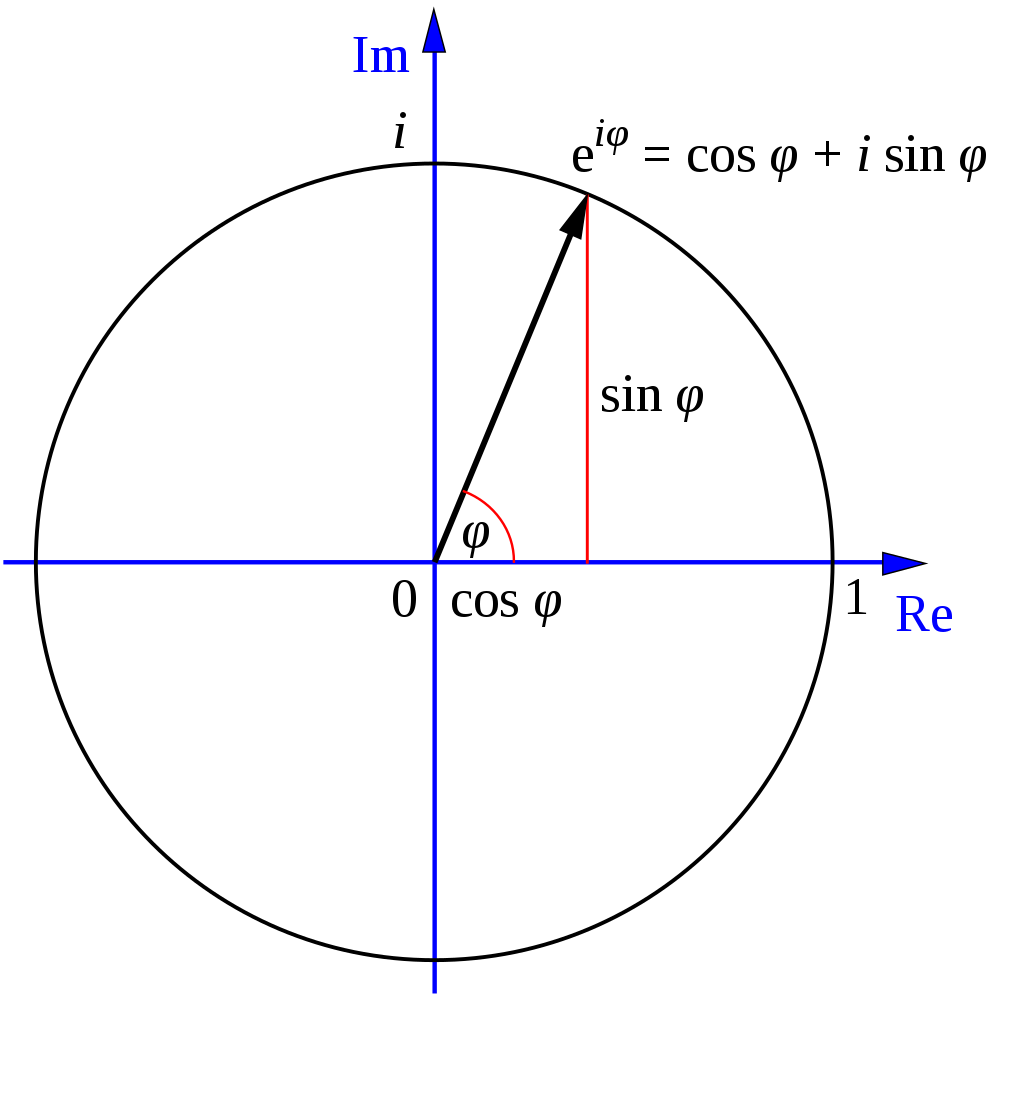
$X_k = $ complex number that represents the amplitude and phase of a periodic function with frequency $\frac{k}{N}$

Euler's Formula

$$\Large e^{ix} = \cos x + i\sin x$$

Adding Periodic Functions

https://betterexplained.com/articles/an-interactive-guide-to-the-fourier-transform/

IFrame('https://betterexplained.com/examples/fourier/?cycles=0,1,1', width=550, height=200)

The circles are our measured values at equally spaced timepoints. We are plotting the real valued portion of each periodic function.

For a given set of function values, how can we determine the periodic functions that sum to those values at those locations?

Getting one timepoint right

IFrame('https://betterexplained.com/examples/fourier/?cycles=1,1,1,1,1', width=550, height=200)

Simply divide up the desired amplitude among the different components.

Not at the origin

"Back up" each cyclic function by changing the phase.

IFrame('https://betterexplained.com/examples/fourier/?cycles=1,1:-90,1:-180,1:-270', width=550, height=200)

Putting it all together...

Treat each data point as it's own "spike" (delta function) and then sum the results. This is what the Fourier transform is doing.

IFrame('https://betterexplained.com/examples/fourier/?time=0,1,2,3', width=550, height=200)

@kalid

Fast Fourier Transformer

An $n \log n$ algorithm (instead of $n^2$).

Can be parallelized.

Many highly optimized implementations, including on GPUs.

2D Fourier Transform

$$\Large X_{u,v} = \sum_{x=0}^{M-1} \sum_{y=0}^{N-1} f(x,y) e^{- i 2\pi \left( \frac{ux}{M}+\frac{vy}{N} \right)}$$

Decomposing our function into periodic functions in both dimensions.

from PIL import Image
img = Image.open('imgs/ollygrey.tiff')
img

import scipy, numpy as np, matplotlib.pyplot as plt
import scipy.fft
dogFFT = scipy.fft.fft2(np.array(img))
vals = np.log(np.absolute(dogFFT))
R = vals.shape[0]//2; C = vals.shape[1]//2;
vals = np.roll(vals, shift=R, axis=0); vals = np.roll(vals, shift=C, axis=1)
plt.matshow(vals)
plt.xticks([0,C,2*C],labels=[-C,0,C]); plt.yticks([0,R,2*R],labels=[-R,0,R])
plt.colorbar()

<matplotlib.colorbar.Colorbar at 0x7ada327da840>

plt.matshow(np.real(scipy.fft.fft2(dogFFT)),cmap='grey')

<matplotlib.image.AxesImage at 0x7ada2fda2d80>

What does each pixel in the FFT transform represent?

def plotFT(u,v):
    Z = np.zeros((512,512))
    Z[u,v] = 1e7
    r = np.real(scipy.fft.ifft2(Z))

    fig = plt.figure(figsize=(20,10))
    ax = fig.add_subplot(2,2,1)
    ax.matshow(r)

    x, y = np.meshgrid(range(512), range(512))
    ax2 = fig.add_subplot(2,1,1,projection='3d')
    ax2.plot_surface(x,y,r)
    return fig

plotFT(0,0);

plotFT(1,0);

plotFT(0,1);

plotFT(1,1);

plotFT(10,5);

Filtering frequencies in the image

def filterFFT(vals,r,invert=False):
    rows, cols = vals.shape[0], vals.shape[1]
    y, x = np.ogrid[:rows, :cols]  # Create grid of indices
    mask =  (np.sqrt((x)**2 + (y)**2) < r) |  (np.sqrt((cols-x)**2 + (rows-y)**2) < r) |  (np.sqrt((cols-x)**2 + (y)**2) < r) |  (np.sqrt((x)**2 + (rows-y)**2) < r) 
    if invert:
        mask = ~mask
    return mask*vals

vals = filterFFT(dogFFT,50)
R = vals.shape[0]//2; C = vals.shape[1]//2
vals = np.roll(vals, shift=R, axis=0); vals = np.roll(vals, shift=C, axis=1)
plt.matshow((np.log(np.absolute(vals))));

/tmp/ipykernel_155314/3483986985.py:4: RuntimeWarning: divide by zero encountered in log
  plt.matshow((np.log(np.absolute(vals))));

plt.matshow(np.real(scipy.fft.fft2(filterFFT(dogFFT,50))),cmap='grey')

<matplotlib.image.AxesImage at 0x7ada1e3e0e30>

plt.matshow(np.real(scipy.fft.fft2(filterFFT(dogFFT,20))),cmap='grey')

<matplotlib.image.AxesImage at 0x7ada2d3ddd00>

High Frequencies

plt.matshow(np.real(scipy.fft.fft2(filterFFT(dogFFT,20,True))),cmap='grey')

<matplotlib.image.AxesImage at 0x7ada1e369910>

plt.matshow(np.real(scipy.fft.fft2(filterFFT(dogFFT,100,True))),cmap='grey')

<matplotlib.image.AxesImage at 0x7ada13be5280>

Holistic Tranform

Everything depends on everything else.

The Phase Problem

Phases

How to get $\phi$

Molecular Replacement

Estimate phases from a homologous known structure (or predicted structure - AlphaFold). Needs to be very similar.

Isomorphous Replacement

Change the diffraction pattern through the addition of a heavy atom to the crystal. This is why you might see some weird atoms in a protein structure (e.g. mercury, uranium). These atoms have such a larger signal they act as "guideposts".

Anomalous Diffraction

Change the wavelength of the X-rays and monitor the change in diffraction. Requires the use of atoms which exhibit anomalous diffraction at appropriate wavelengths. This is why you might see the sulfur replaced with selenium in methionine/cysteine.

Molecular Animal Replacement

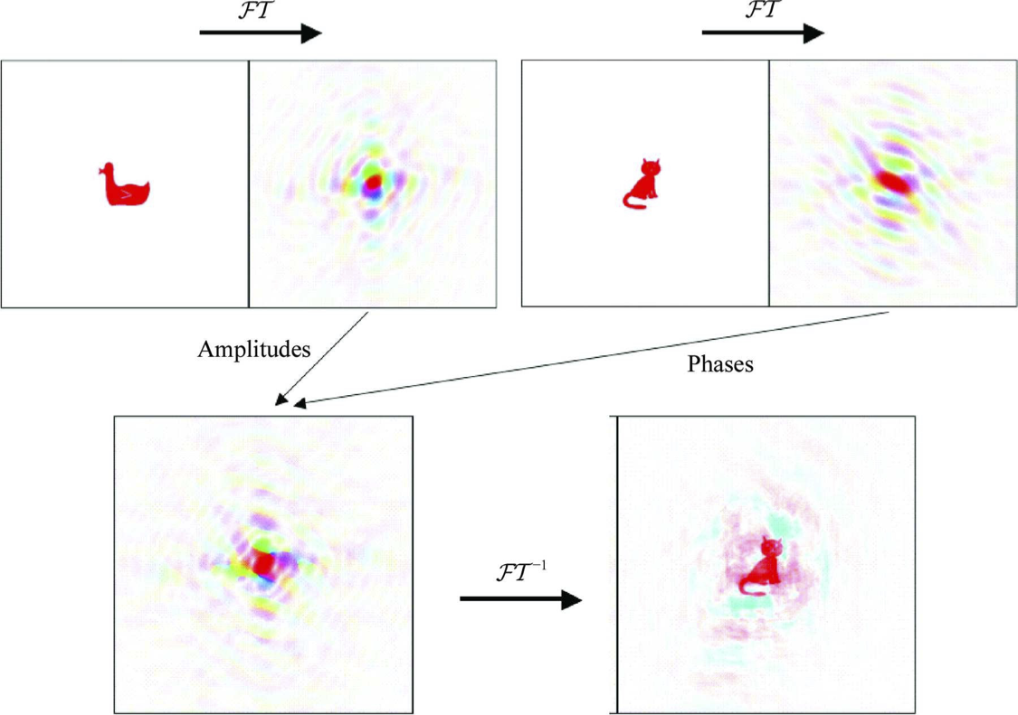
^{Taylor GL. Introduction to phasing. Acta Crystallographica Section D: Biological Crystallography. 2010 Apr 1;66(4):325-38.}

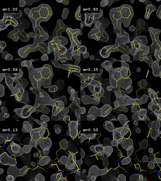
Phase Error Effect

Effect on electron density as correct phases (m=1.0) are corrupted with phases from a random structure.

Phases are iteratively improved

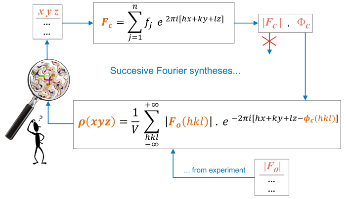
$f_j$ is the atom scattering factor and is dependent on the atom type, position ($xyz$) and thermal factor ($B$).

Step 4: Refine Model

Optimize atomic parameters (x, y, z, B) in order to minimize the sum of squared differences between observed and calculated structure factor amplitudes:

$$E = \sum_{hkl} \left( |F_o| - |F_c|_{xyzB} \right)^2$$

$x,y,z,B$ are free parameters in this optimization process, but there are physical contraints on realistic atom positions (e.g., they must be connected amino acids in the right sequence with reasonable bond lengths and angles).

Hence "fudge factor" $B$ (accounts for anything that would smear the electron density - thermal vibrations, larger movements, crystal defects).

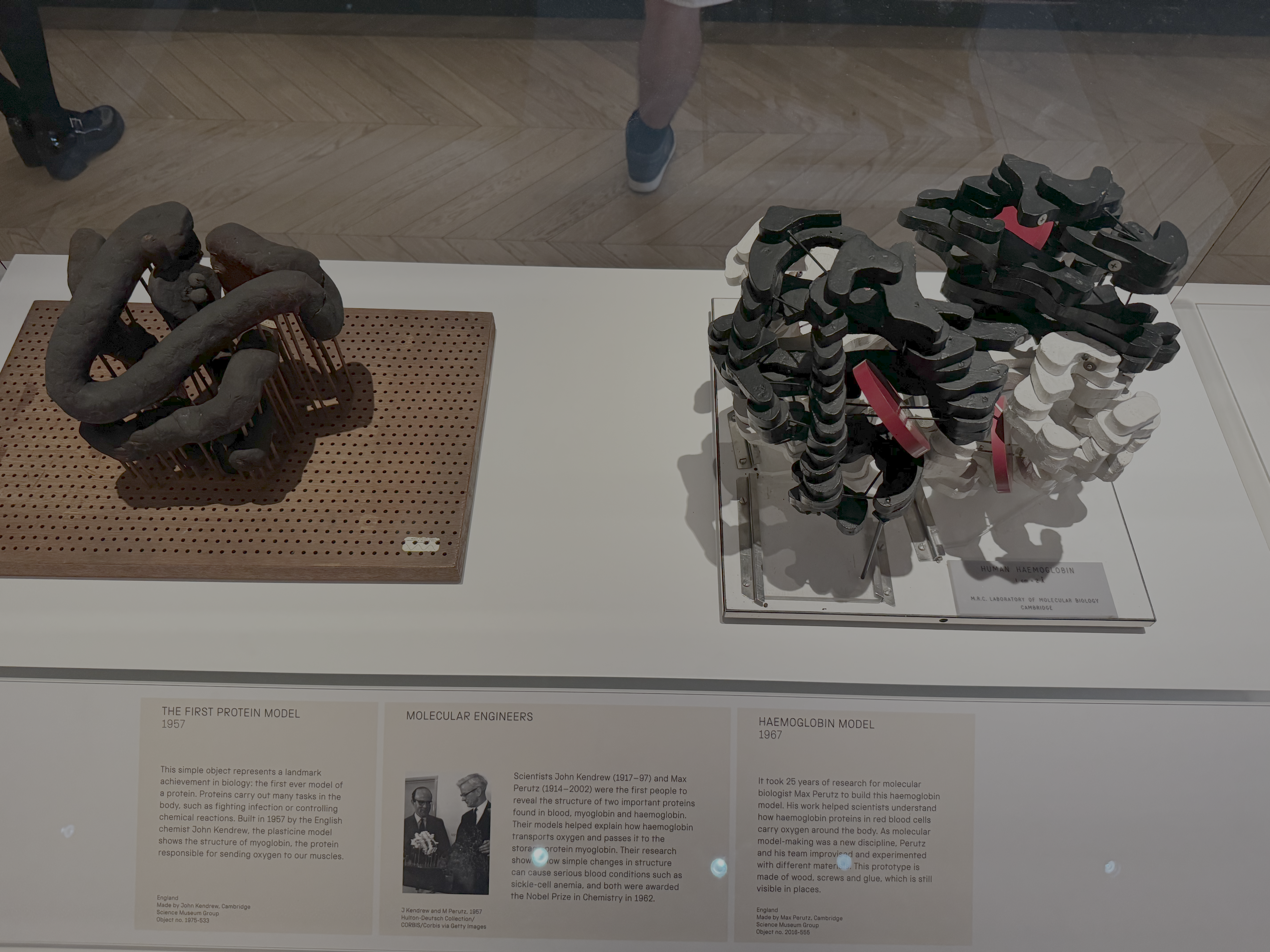
The first protein structure

Refinement

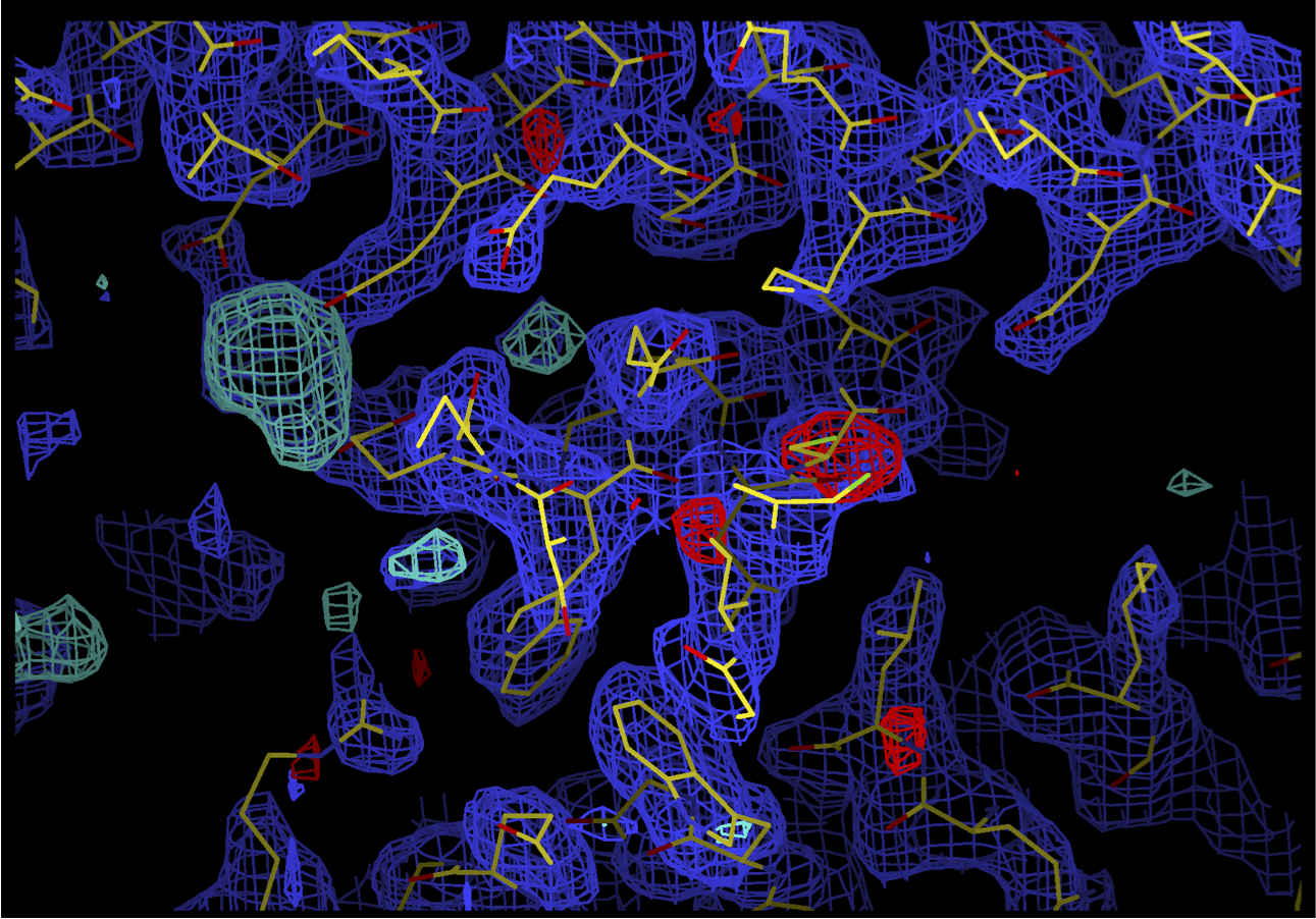
Model (atom positions) is typically fit to 2fofc map: $2|F_o|-|F_c|$

Model refinement is not necessarily fully automated. Difference maps are inspected and coordinates manually updated (but there will always be noise).

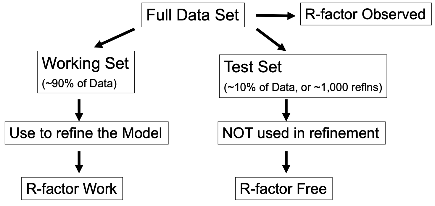
Model Quality: R-value

Asses how close calculated diffraction map is to observed.

$$ R = \frac{\sum_{hkl} \left| |F_o| - |F_c| \right|}{\sum_{hkl} |F_o|}$$

Random structure has $R \approx .6$

Typically end up with $R \approx .2$

This looks very similar to what we are optimizing for. What's the problem with this?

Omit Maps

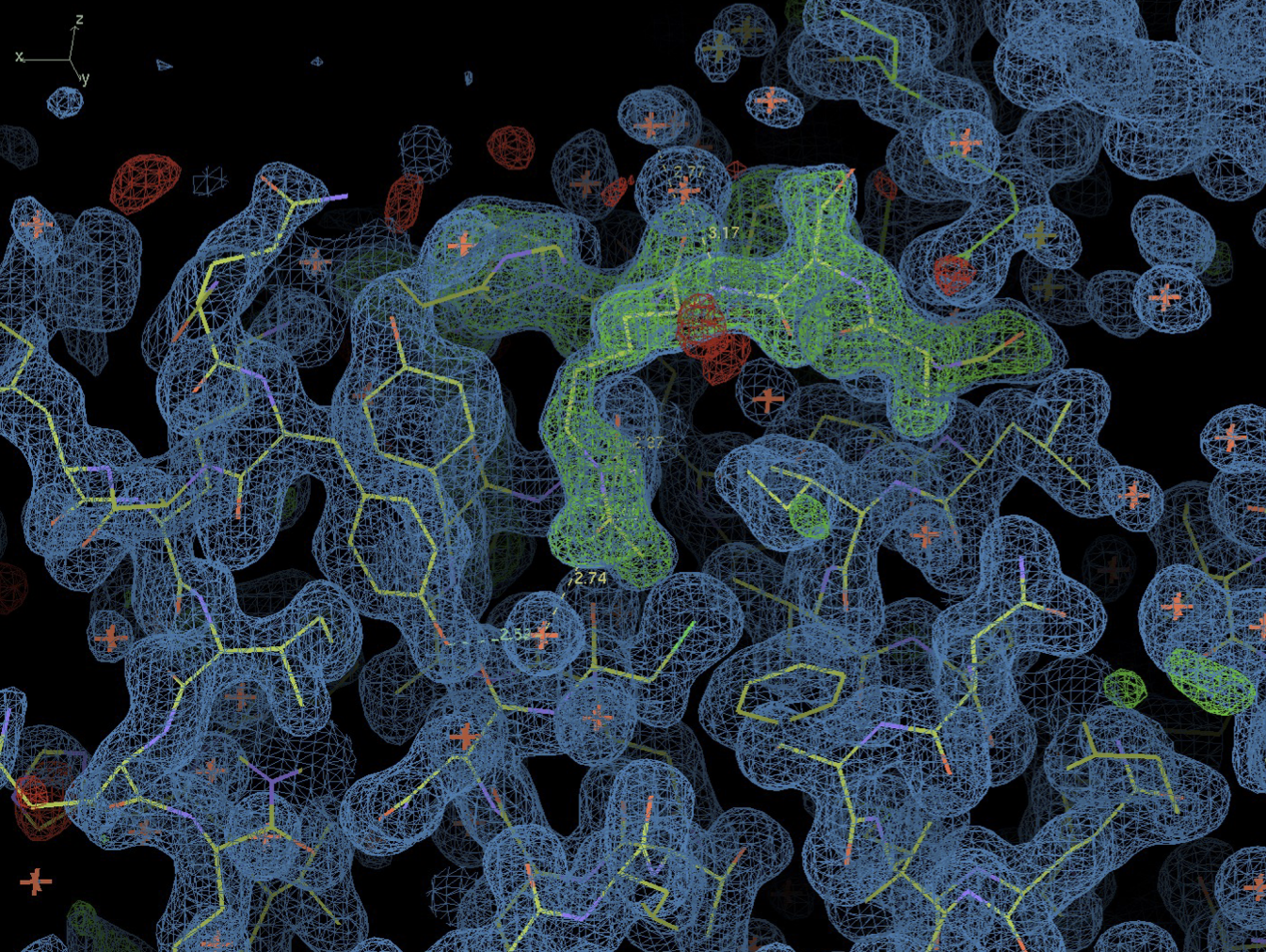
The R-score is comparing the model to experimental data in reciprocal space. We can do something similar in real space.

ALTLOC

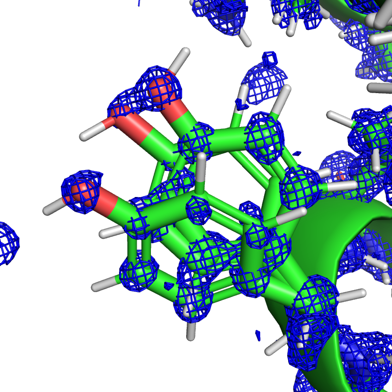
Sometimes multiple locations for the same atom best explains the elctron density. In these cases, the crystallographer will provide alternative locations.

PDB: 1EJG. Resolution 0.54A.

Missing Atoms

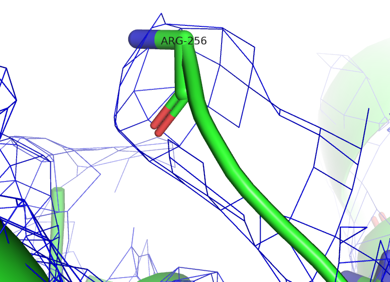
If there isn't enough electron density to place atoms, they may be omitted entirely.

PDB: 1A37. Resolution 3.6A.

Further Validation

Compare model to expected distribution of properties.

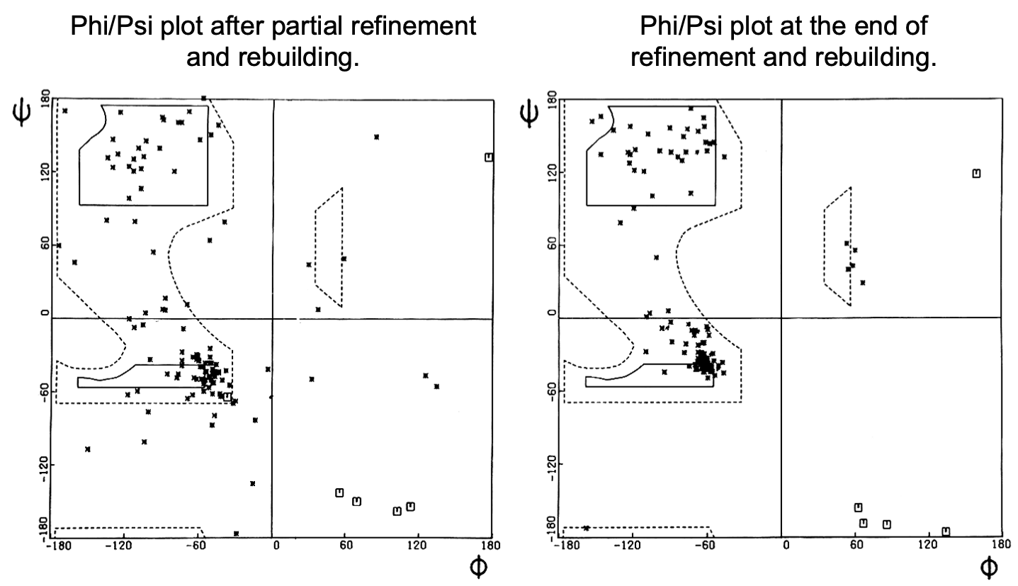
Futher Validation

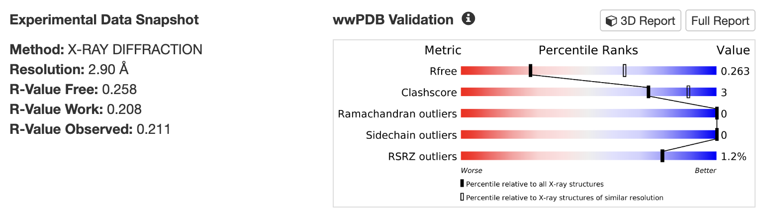
RSRZ: Real space R-value - the percentage of residues that do not fit their electron density well.

Recap

Atoms

There may be missing atoms or extra atoms (alternative locations). Some elements (heavy metals, selenium) may be there for the crystallographer and not be biological.

Resolution

Average measure of quality of data

R-Value

Average measure of quality of model fit to the data.

B-factors

Local measure of quality(?) of electron density.

B-Factors

v = py3Dmol.view(query='pdb:1ycr'); colorB = {'colorscheme':{'prop':'b','gradient':'rwb','min':0,'max':60}}; v.setStyle({'cartoon': colorB, 'stick': colorB});v.show()

3Dmol.js failed to load for some reason. Please check your browser console for error messages.

%%html
<div id="bfactorcol" style="width: 500px"></div>
<script>
    var divid = '#bfactorcol';
	jQuery(divid).asker({
	    id: divid,
	    question: "In the previous figure, which color residues are moving more according to the B factors?",
		answers: ["Red","Blue"],
        server: "https://bits.csb.pitt.edu/asker.js/example/asker.cgi",
		charter: chartmaker})
    
$(".jp-InputArea .o:contains(html)").closest('.jp-InputArea').hide();


</script>

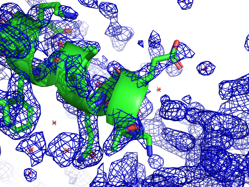
Electron Density Maps

The best measure of local quality is the electron density map itself.

Unfortunately, the map isn't always available, but when it is can easily fetch PDB,type=2fofc (e.g. fetch 1cll, type=2fofc). May have to manually download from https://www.ebi.ac.uk/emdb/

%%html
<iframe width="700" height="500" src="https://3dmol.csb.pitt.edu/tests/auto/generate_test.cgi?test=test_isosurface_coords" frameborder="0" allow="accelerometer; autoplay; clipboard-write; encrypted-media; gyroscope; picture-in-picture" allowfullscreen></iframe>

NMR Structure Determination

Makes X-ray Crystallography Look Easy

Nuclear magnetic resonance spectroscopy

The principle of NMR usually involves three sequential steps:

1. The alignment (polarization) of the magnetic nuclear spins in an applied, constant magnetic field $B_0$.
2. The perturbation of this alignment of the nuclear spins by a weak oscillating magnetic field, usually referred to as a radio-frequency (RF) pulse.
3. Detection and analysis of the electromagnetic waves emitted by the nuclei of the sample as a result of this perturbation.

--Wikipedia

Spin

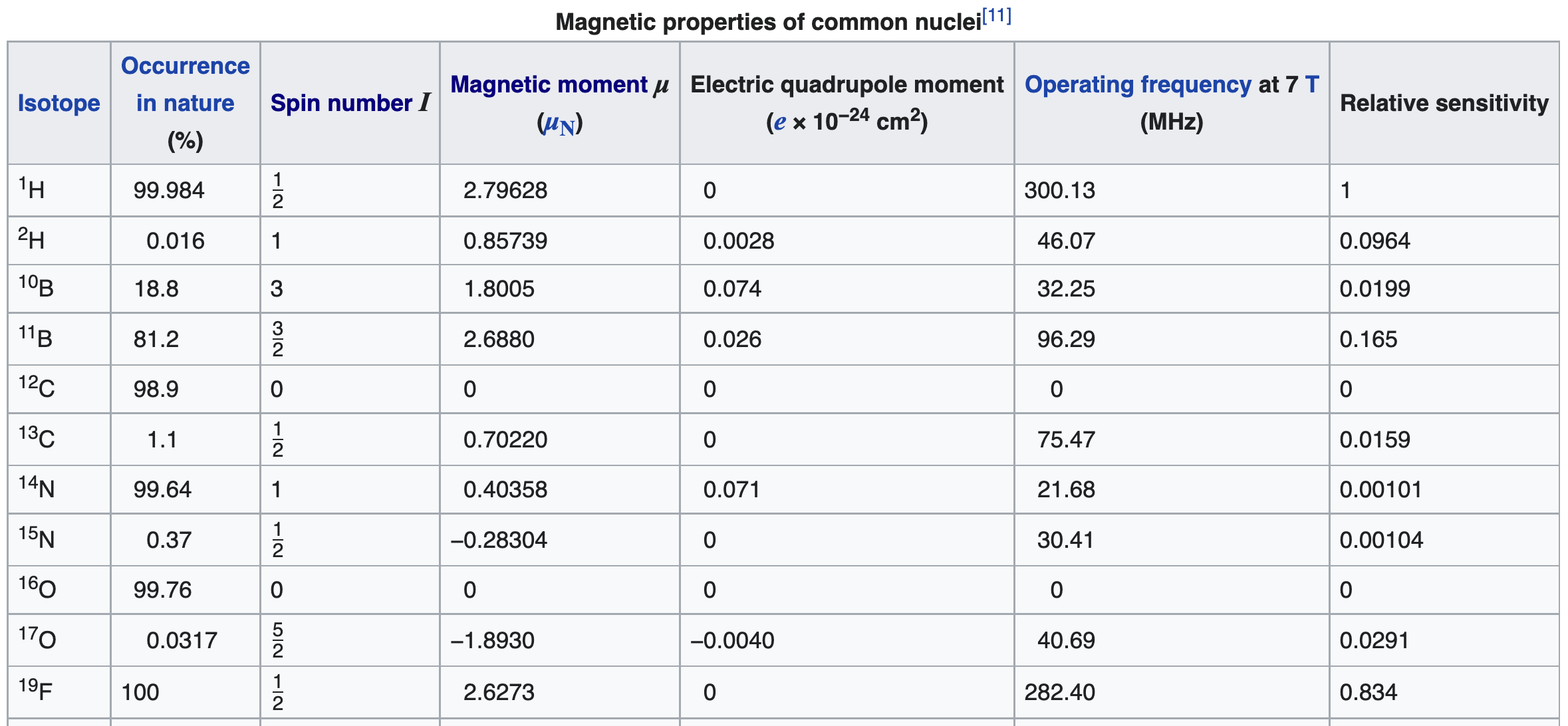
Only some nuclei are suitable for NMR ($\mathrm{^1H, ^{13}C, ^{15}N}$ most relevant to proteins)

Chemical Shifts

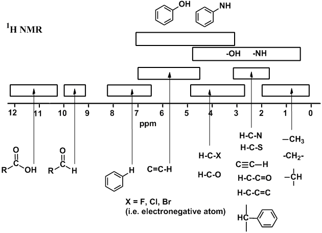
The exact resonant frequency of a nucleus depends on the local environment (nearby atoms, bond lengths/angles, etc).

The difference in resonance frequency compared to a reference due to this local environment is the chemical shift.

Each chemical shift gives us a tiny bit of information about the structure.

2D NMR

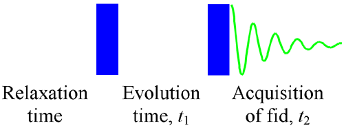
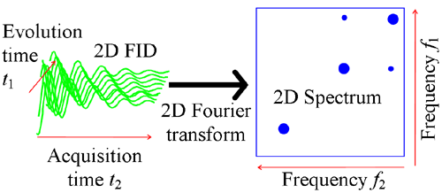
Instead of a single pulse, two pulses are used. Spectra are collected for different evolution times and a 2D Fourier transform computed.

Off-diagonal peaks indicate interactions.

^{http://chem.ch.huji.ac.il/nmr/techniques/2d/2d.html}

Correlation spectroscopy (COSY)

Cross-peaks indicate magnetization transfer between coupled atoms.

Atoms that are 2,3, or 4 bonds away.

Nuclear Overhauser effect spectroscopy (NOESY)

Nuclear Overhauser effect (NOE) is the transfer of nuclear spin polarization.

Identifies atoms that are near in space (not in bond distance).

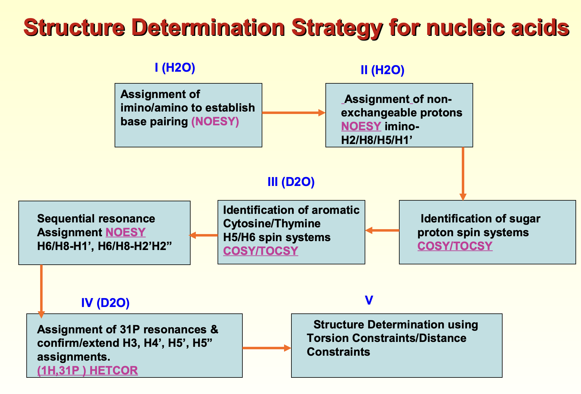^{https://www.tifr.res.in/~iupab/2d-learning-WS2009-new.pdf}

Restraints

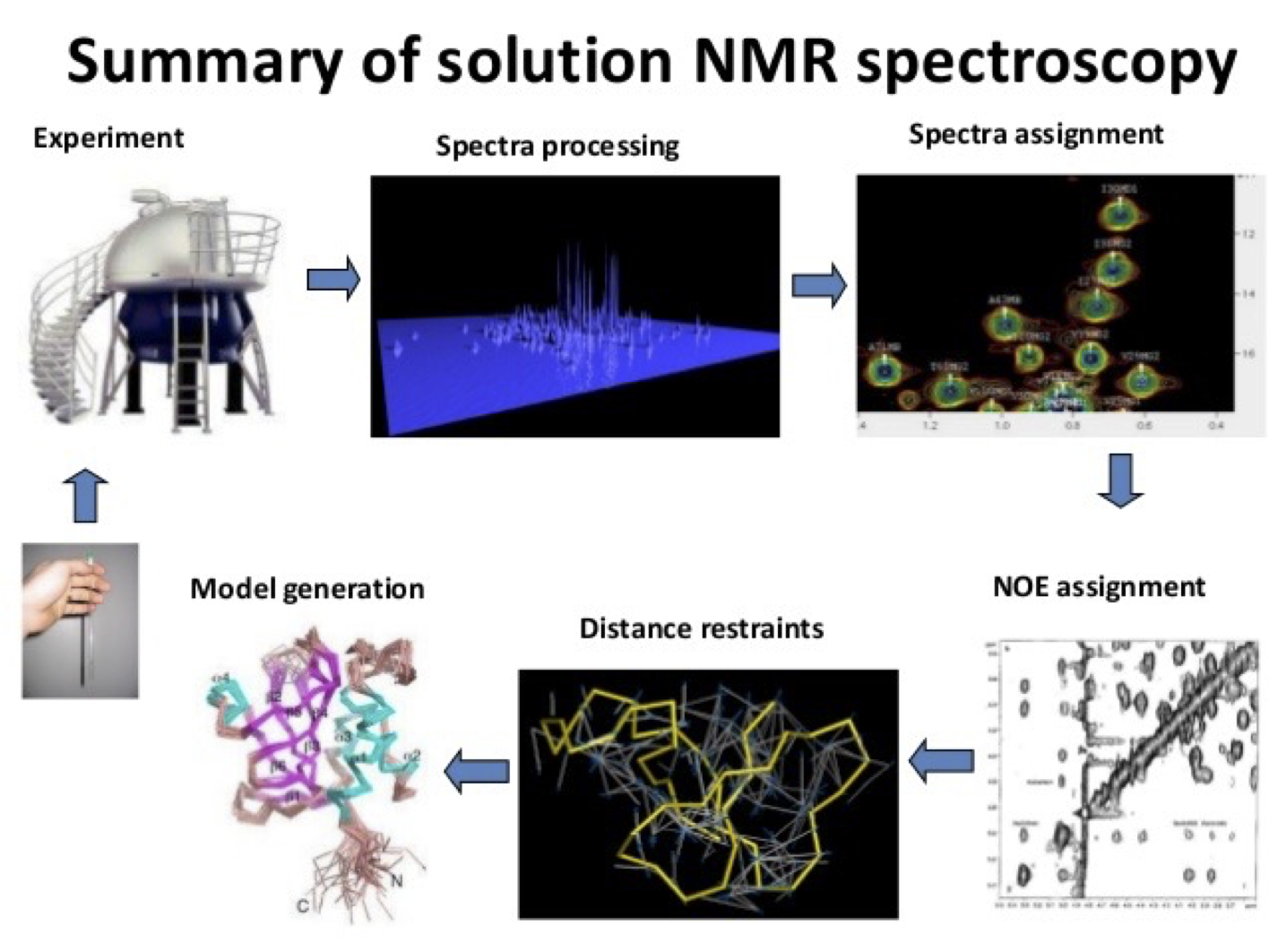
All the collected NMR data is assembled to create a collection of restraints:

• Distance restraints (mostly NOESY)
• Angle restraints (coupling)
• Orientation restraints

No restraints are exact - they represent a distribution of structures.

Model Generation

These restraints, along with physical requirements, are used to generate an ensemble of models that are consistent with the restraints.

import prody
prody.showProtein(prody.parsePDB('1pfl')).show()

3Dmol.js failed to load for some reason. Please check your browser console for error messages.

Validation

Model structures are compared to expected distributions of angles and interactions.

NMR Can Map Binding Sites

Krishnamoorthy J, Yu VC, Mok YK. Auto-FACE: an NMR based binding site mapping program for fast chemical exchange protein-ligand systems. PloS one. 2010 Feb 18;5(2):e8943.

Cryogenic electron microscopy (Cryo EM)

So Cold It's Hot

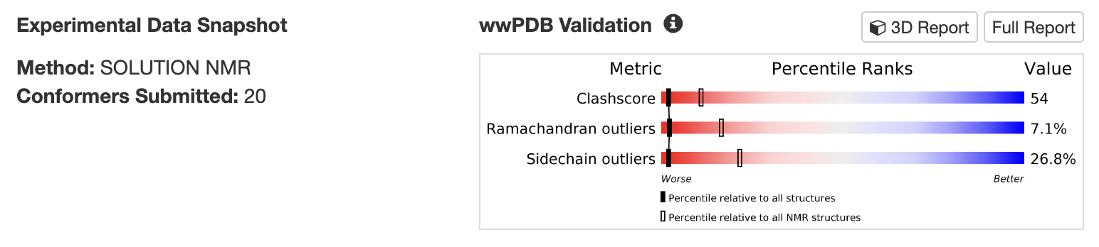
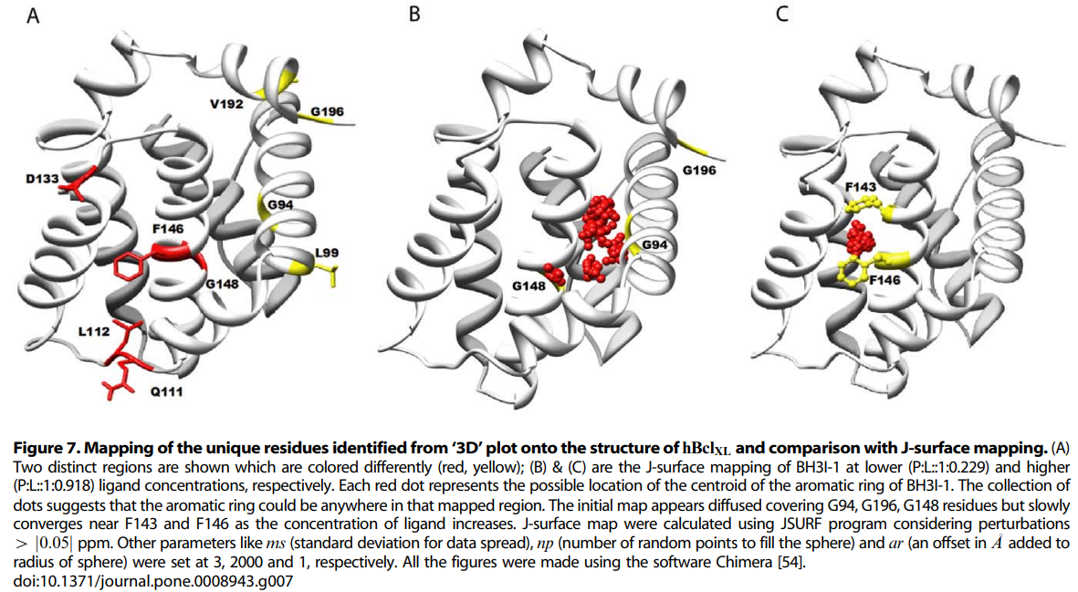
Cryogenic electron tomography (Cryo ET)

Looks at one object from multiple angles. Generally does not achive atomic resolution.

Single Particle Cryo EM

^{https://www.nature.com/articles/d41586-020-00341-9}

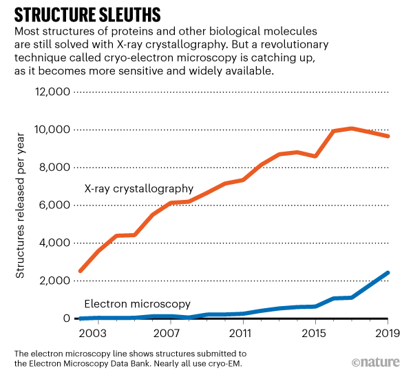
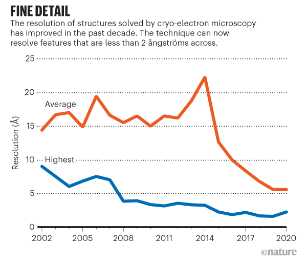
from IPython.display import YouTubeVideo
YouTubeVideo('BJKkC0W-6Qk', width=800, height=300)

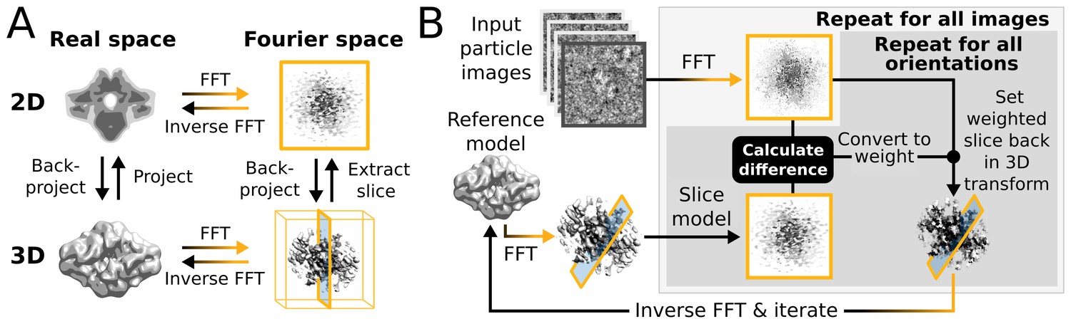
^{Kimanius D, Forsberg BO, Scheres SH, Lindahl E. Accelerated cryo-EM structure determination with parallelisation using GPUs in RELION-2. elife. 2016;5.}

$$\Large \mathcal{F}\left\{f \star g\right\} = \overline{\mathcal{F} \left\{f\right\}} \cdot \mathcal{F}\left\{g\right\}$$

Cross-correlation

Fourier Shell Correlation

Split the data in half - how well does the reconstruction from one half correlate with the other at different frequiencies in frequency space? This is where the resolution comes from.

https://www.nature.com/articles/s42003-023-05724-y

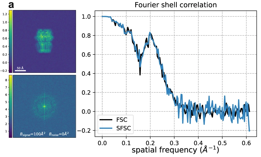
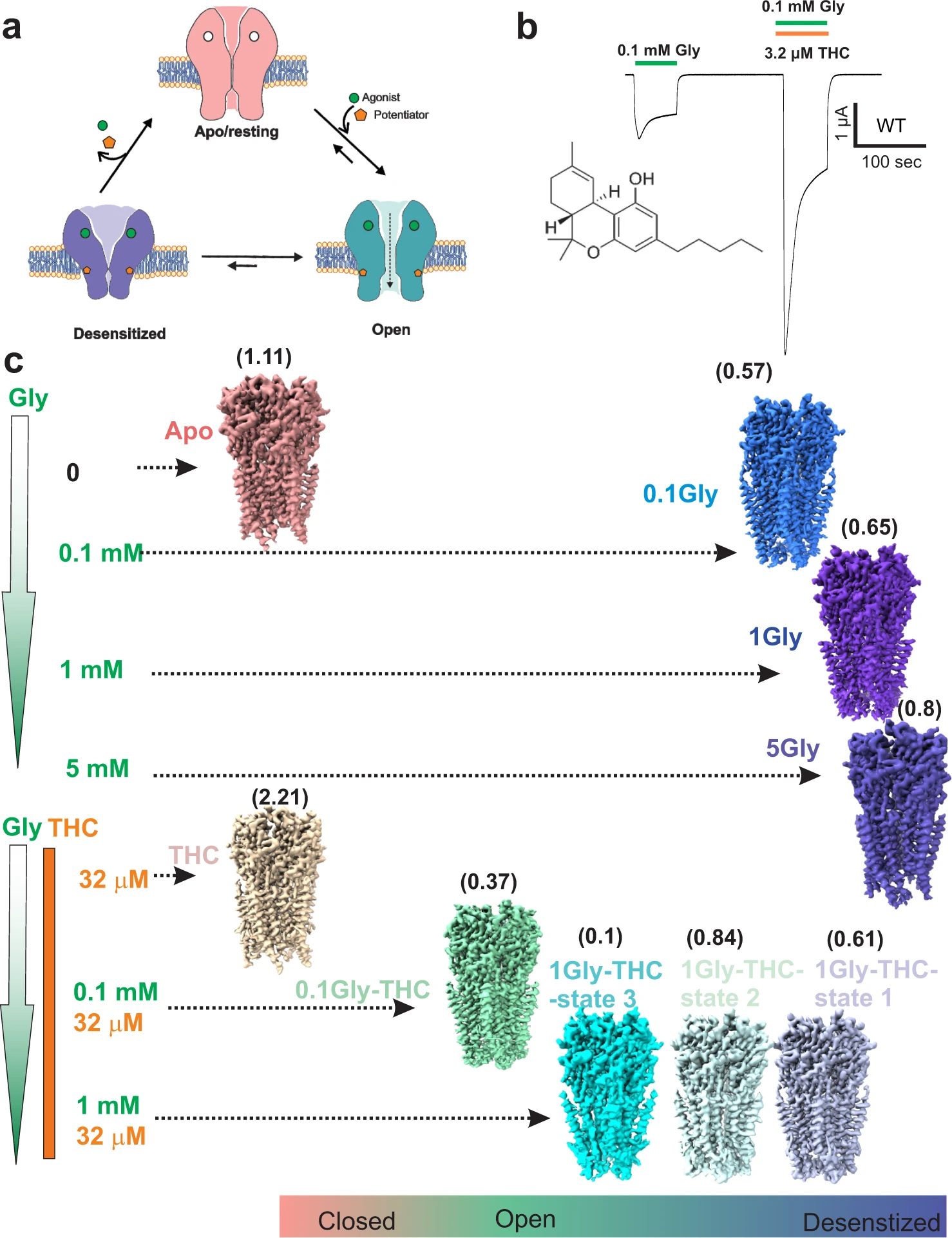Modern computational methods can deconvolve different conformational states.

https://www.nature.com/articles/s41467-022-32594-5

Validation

Check the resolution!

7V2C

1D3E

%%html
<div id="whichmethod" style="width: 500px"></div>
<script>
    var divid = '#whichmethod';
	jQuery(divid).asker({
	    id: divid,
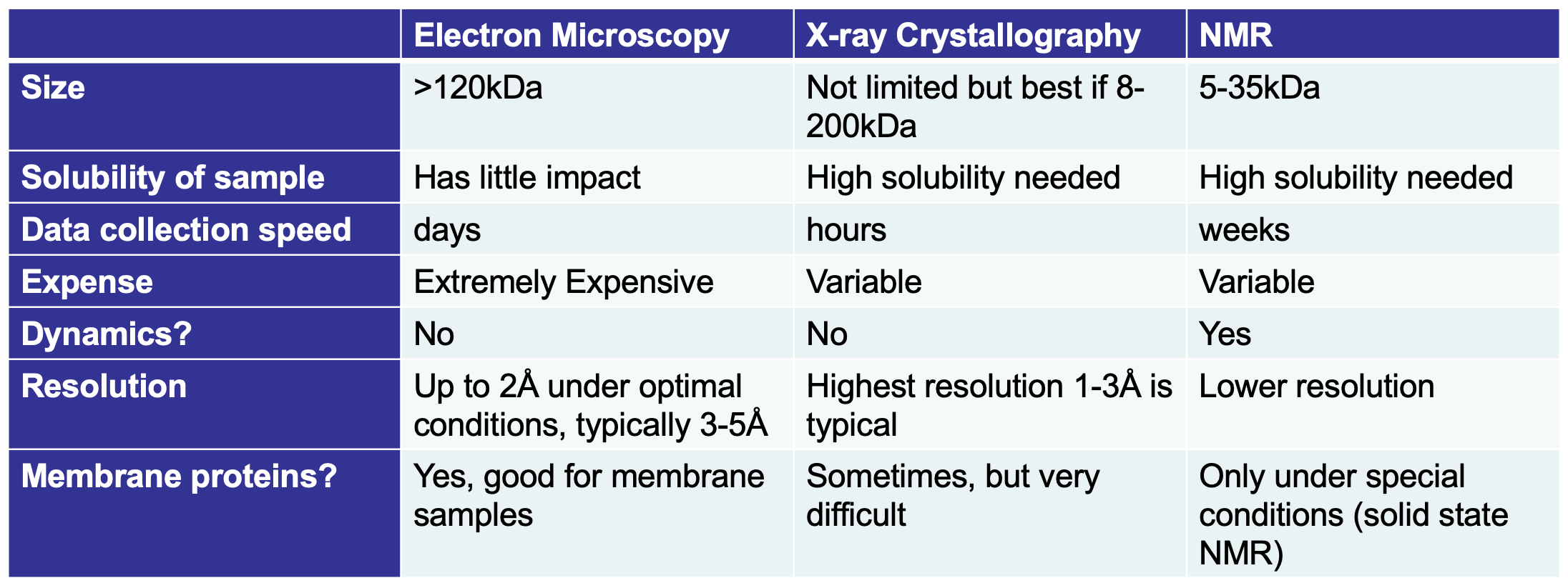
	    question: "Which method least respects biological conditions?",
		answers: ["X-Ray","NMR","CryoEM"],
        server: "https://bits.csb.pitt.edu/asker.js/example/asker.cgi",
		charter: chartmaker})
    
$(".jp-InputArea .o:contains(html)").closest('.jp-InputArea').hide();


</script>

%%html
<div id="whichmethod2" style="width: 500px"></div>
<script>
    var divid = '#whichmethod2';
	jQuery(divid).asker({
	    id: divid,
	    question: "Which method provides the most information about protein dynamics?",
		answers: ["X-Ray","NMR","CryoEM"],
        server: "https://bits.csb.pitt.edu/asker.js/example/asker.cgi",
		charter: chartmaker})
    
$(".jp-InputArea .o:contains(html)").closest('.jp-InputArea').hide();


</script>

Recitation - Cluster Usage and Setp

Assignment 1 - Due Friday