%%html
<script src="https://bits.csb.pitt.edu/preamble.js"></script>
The Plan
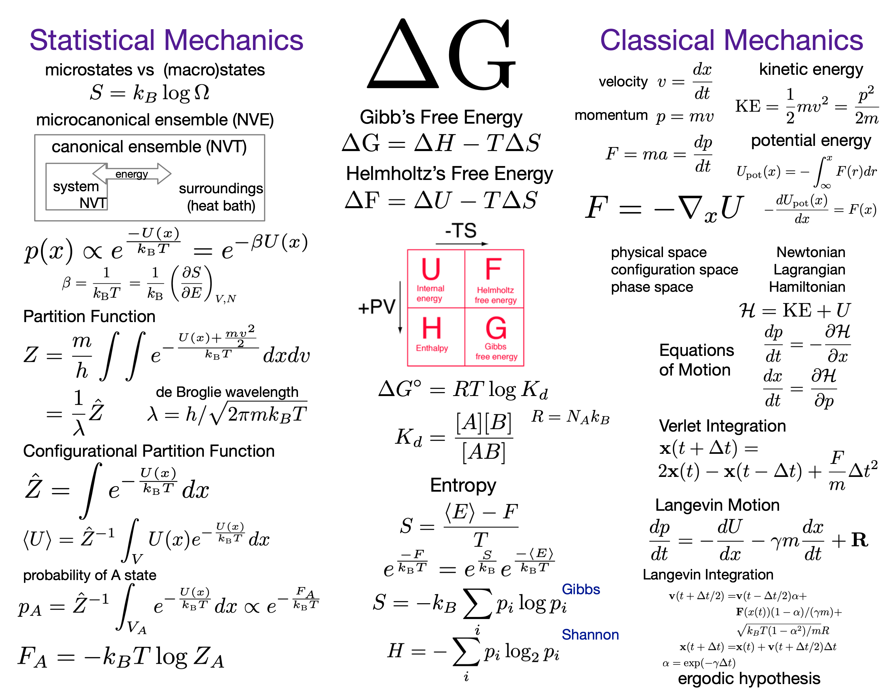
The Harmonic Oscillator
By Svjo - Previously uploaded version of Animated-mass-spring.gif here, CC BY-SA 3.0, Link
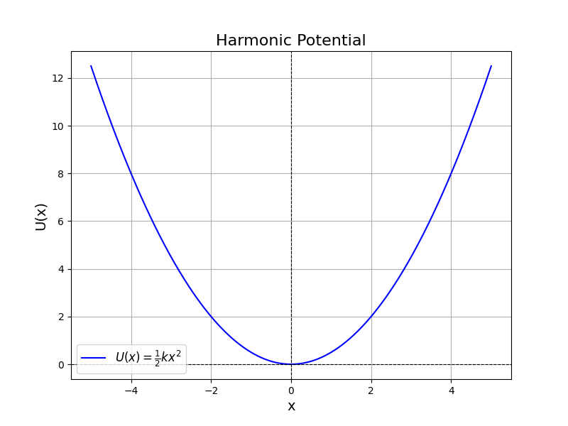
$$\Large U(x) = U_0 + \frac{1}{2} k (x-x_0)^2$$
where $U_0$ is the baseline potential energy, $k$ is the spring constant and $x_0$ is the center position.
%%html
<div id="sprintk" style="width: 500px"></div>
<script>
    var divid = '#sprintk';
	jQuery(divid).asker({
	    id: divid,
	    question: "What happens to the potential well as you increase the spring constant k?",
		answers: ["Gets narrower","Gets wider",'Moves up',"Moves down"],
        server: "https://bits.csb.pitt.edu/asker.js/example/asker.cgi",
		charter: chartmaker})

$(".jp-InputArea .o:contains(html)").closest('.jp-InputArea').hide();


</script>
Configuration vs Phase Space
%%html
<div id="phasedim" style="width: 500px"></div>
<script>
    var divid = '#phasedim';
	jQuery(divid).asker({
	    id: divid,
	    question: "How many dimensions does the phase space of a molecule with N atoms have?",
		answers: ["2N","3N","6N","N^3",'2N^3'],
        server: "https://bits.csb.pitt.edu/asker.js/example/asker.cgi",
		charter: chartmaker})

$(".jp-InputArea .o:contains(html)").closest('.jp-InputArea').hide();


</script>
Newtonian
$$\Large F = - \frac{\partial U(x)}{\partial x} = - \frac{\partial}{\partial x} \left( U_0 + \frac{1}{2}kx^2 \right) = -kx$$ $$\Large F = ma = \frac{dp}{dt} = \frac{d}{dt} mv = \frac{d}{dt} m \frac{dx}{dt} = m\frac{d^2x}{dt^2}$$
$$\Large m\frac{d^2x}{dt^2} = -kx$$ This is the equation of motion for an object attached to a spring. The solution to this second order differential equation tells us how the system evolves.
Hamiltonian
$$\Large H = \mathrm{KE} + U = \frac{1}{2}\frac{p^2}{m} + \frac{1}{2}kx^2$$
$$\frac{dp}{dt} = - \frac{\partial H}{\partial x} = - \frac{\partial \left( \frac{1}{2}\frac{p^2}{m} + \frac{1}{2}kx^2\right)} {\partial x} = -kx $$ $$\frac{dx}{dt} = \frac{\partial H}{\partial p} = \frac{\partial \left( \frac{1}{2}\frac{p^2}{m} + \frac{1}{2}kx^2\right)} {\partial p} = \frac{p}{m}$$
We have a system of first order differential equations that tell us how the system evolves. If we solve for $\frac{dp}{dt}$ and substitute, we get our second order equations of motion.
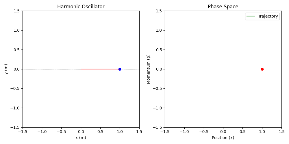
Solution
What function satisfies this relationship?
$$m\frac{d^2x}{dt^2} = -kx$$
$$x(t) = A\cos(\omega t) + B \sin(\omega t)$$ where $$\omega = \sqrt{\frac{k}{m}} \\ A = x(0) \\ B = w^{-1}\frac{dx(0)}{dt}$$
mass = 1.0; k = 1.0
omega = np.sqrt(k / mass)
x0 = 1.0  # Initial position
v0 = 0  # Initial velocity

# Time settings
time_step = 0.02  # Time step (s)
total_time = 20.0  # Total simulation time (s)
times = np.arange(0, total_time, time_step)

# Solve the equations of motion
positions = x0 * np.cos(omega * times) + (v0 / omega) * np.sin(omega * times)
velocities = -x0 * omega * np.sin(omega * times) + v0 * np.cos(omega * times)
plt.figure(figsize=(10,4))
plt.plot(times,positions,label='$x(t)$')
plt.plot(times,velocities,label='$v(t)$')
plt.legend(); plt.xlabel('t')
Text(0.5, 0, 't')

%%html
<div id="harmmicro" style="width: 500px"></div>
<script>
    var divid = '#harmmicro';
	jQuery(divid).asker({
	    id: divid,
	    question: "What can be said about the probabilities of the microstates (positions in phase space) of this system?",
		answers: ["They are equal","Equal excluding extrema","Variable"],
        server: "https://bits.csb.pitt.edu/asker.js/example/asker.cgi",
		charter: chartmaker})

$(".jp-InputArea .o:contains(html)").closest('.jp-InputArea').hide();


</script>
Let's heat things up!
Boltzmann Distribution
The Boltzmann distribution converts the energy landscape of a system into a probability distribution
$$\Large \rho(x) \propto e^{\frac{-U(x)}{k_B T}}$$
$k_B= 1.4\times 10^{-23} \,\mathrm{J\,K}^{-1}$ is Boltzmann constant

%%html
<div id="boltz1" style="width: 500px"></div>
<script>
    var divid = '#boltz1';
	jQuery(divid).asker({
	    id: divid,
	    question: "Higher energy microstates are",
		answers: ["More probable","Less Probable","Depends"],
        server: "https://bits.csb.pitt.edu/asker.js/example/asker.cgi",
		charter: chartmaker})

$(".jp-InputArea .o:contains(html)").closest('.jp-InputArea').hide();


</script>
%%html
<div id="boltz2" style="width: 500px"></div>
<script>
    var divid = '#boltz2';
	jQuery(divid).asker({
	    id: divid,
	    question: "As temperature increases, higher energy microstates will become",
		answers: ["More probable","Less Probable","Depends"],
        server: "https://bits.csb.pitt.edu/asker.js/example/asker.cgi",
		charter: chartmaker})

$(".jp-InputArea .o:contains(html)").closest('.jp-InputArea').hide();


</script>
Harmonic Partition Function
The normalization factor for the Boltzmann distribution is called the Partition Function
$$\Large \rho(x)= \frac{ e^{-U(x)/k_B T} }{\int_V \,e^{-U(x)/k_B T}dx }$$
$$ \int_V \rho(x) = 1$$
$$\Large \hat{Z}\equiv \int_V \,e^{-U(x)/k_B T} dx = \lambda Z$$
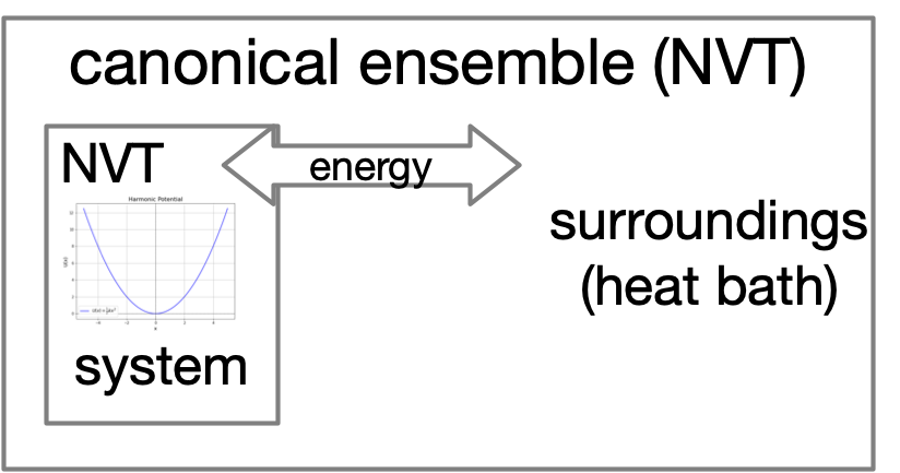
Ensemble Properties
We can compute mean of any property of states (defined by function $g$) using the defition of expectation.
$$\Large \langle g \rangle = \int_V \,g(x)\,\rho(x) dx \\ \Large \langle g \rangle = \frac{\int_V g(x)\, e^{-U(x)/k_B T}dx}{\hat{Z}} $$
Average Energy of Harmonic System
$$\Large U_{\mathrm{harm}}= U_0 + \left( \frac{\kappa}{2}\right)(x-x_0)^2 $$
$$\Large \langle U_{\mathrm{harm}} \rangle = \frac{\int_V U_{\mathrm{harm}}(x)\, e^{-U_{\mathrm{harm}}(x)/k_B T}dx} {\int_V e^{-U_{\mathrm{harm}}(x)/k_B T}dx}$$
What is $\hat{Z}$?
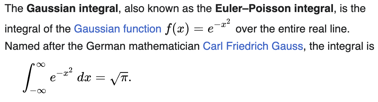
Partition Function of Harmonic Potential
$$\Large \hat{Z}_{\mathrm{harm}}= \int_V e^{-\left ( U_0 + \left( \frac{\kappa}{2}\right)(x-x_0)^2 \right)/k_B T}dx \\ \Large \hat{Z}_{\mathrm{harm}}= e^{-U_0/k_B T}\int_{-\infty}^{\infty} e^{-\frac{\kappa (x-x_0)^2}{2k_B T}dx} = e^{-U_0/k_B T}\sqrt{\frac{2\pi k_B T}{\kappa}}$$
Average Energy
$$\Large \langle U_{\mathrm{harm}} \rangle = \frac{\int_V U_{\mathrm{harm}}(x)\, e^{-U_{\mathrm{harm}}(x)/k_B T}dx} {\int_V e^{-U_{\mathrm{harm}}(x)/k_B T}dx}$$
This can be solved exactly (using additional integration identities) $$\Large \langle U_{\mathrm{harm}}\rangle= U_0 + \frac{1}{2}k_BT$$
This is the equipartition theorem. Any coordinate whose energy depends quadratically on its value (e.g., velocity $= 1/2 mv^2$) will have an average energy of $\frac{1}{2}k_BT$.
Each degree of freedom that appears quadratically in the expression for the total energy contributes an average energy of $\frac{1}{2}k_BT$ to the system
States
Biomolecules have an essentially infinite set of configurations. We are interested in the sets of configurations that behave in a “similar way.” States represent a way to cluster configurations of biomolecules by function.

- What are the relative probabilities to observe molecule in state A vs. state B?
- What properties affect these probabilities?
State Probabilties
$$ p_A = \hat{Z}^{-1}\int_{V_A} e^{-U(x)/k_B T} dx \approx \hat{Z}^{-1}\int_{\infty}^{\infty} e^{-U_A(x)/k_B T} dx \\ p_B = \hat{Z}^{-1}\int_{V_B} e^{-U(x)/k_B T dx} \approx \hat{Z}^{-1}\int_{\infty}^{\infty} e^{-U_B(x)/k_B T dx}$$
The ratio of probabilties is given by:
$$\Large \frac{p_A}{p_B} = \frac{\int_{V_A} e^{-U(x)/k_B T}dx} {\int_{V_B} e^{-U(x)/k_B T} dx} \approx \sqrt{\frac{\kappa_b}{\kappa_a}}$$
%%html
<div id="harmstate1" style="width: 500px"></div>
<script>
    var divid = '#harmstate1';
	jQuery(divid).asker({
	    id: divid,
	    question: "In this diagram, which state is more probable?",
		answers: ["A","B","Neither"],
        server: "https://bits.csb.pitt.edu/asker.js/example/asker.cgi",
		charter: chartmaker})

$(".jp-InputArea .o:contains(html)").closest('.jp-InputArea').hide();


</script>
Free Energy of a State
$$\Large \frac{p_A}{p_B} = \frac{\int_{V_A} dx\, e^{-U(x)/k_B T}} {\int_{V_B} dx\, e^{-U(x)/k_B T}} \equiv \frac{e^{-F_A/k_B T}} {e^{-F_B/k_B T}}$$
In general for a state $i$ we have
$$\Large F_i = -k_B T \ln \left( {{Z_i}}\right)$$
This is we call the free energy of state $i$.
The probability distribution of states follows the Boltzmann distribution in free energy $p_i \propto e^{-F_i/k_BT}$
Free Energy of Harmonic Well
$$\Large U(x)= U_i + \left( \frac{\kappa_i}{2}\right)(x-x_i)^2$$
$$\Large \hat{Z}=\int_{V_i} dx\,e^{-U_i/k_BT - \frac{1}{2}\kappa_i(x-x_i)^2/k_B T} = e^{-U_i/k_BT}\sqrt{\frac{2\pi k_B T}{\kappa_i}}$$ $$\Large F_i = U_i - k_B T \ln \left(\lambda^{-1}\sqrt{\frac{2\pi k_B T}{\kappa_i}}\right)$$
Entropy
$$\Large S\equiv \frac{\langle E\rangle - F}{T}$$ $$\left( S = \frac{ \langle K\rangle + \langle U\rangle - F}{T}= \frac{k_B}{2} + \frac{\langle U\rangle - F}{T} \right)$$
Alternatively: $$\Large F = \langle E \rangle - TS$$
The probability of a state $i$ can then be written $$\Large p_i \propto e^{-F_i/k_B T}= e^{+S_i/k_B} e^{-\langle E\rangle_i /k_B T}$$
The Boltzmann factor for a state is just the Boltzmann factor for its average energy times a factor, which will turn out to be related to volume in configuration space (or number of states in a discrete space).
Summary
| Microstate = single configuration | Macrostate = set of configurations | |
|---|---|---|
| Partition function | - | $ \hat{Z}= \int_V e^{-U(x)/k_BT} dx$ |
| Configuration energy | $U(x)$ | $\langle U \rangle = \hat{Z}^{-1} \int_V U(x)\,e^{-U(x)/k_B T} dx$ |
| Relative probability | $e^{-U(x)/k_B T}$ | $e^{-F/k_B T} \propto e^{S/k_B}\,e^{-\langle U \rangle/k_B T}$ |
| Free energy | - | $F = - k_B T \ln Z$ |
| Entropy | - | $S = \frac{k_B}{2} + \frac{\langle U\rangle-F}{T} $ |
Double square well potential
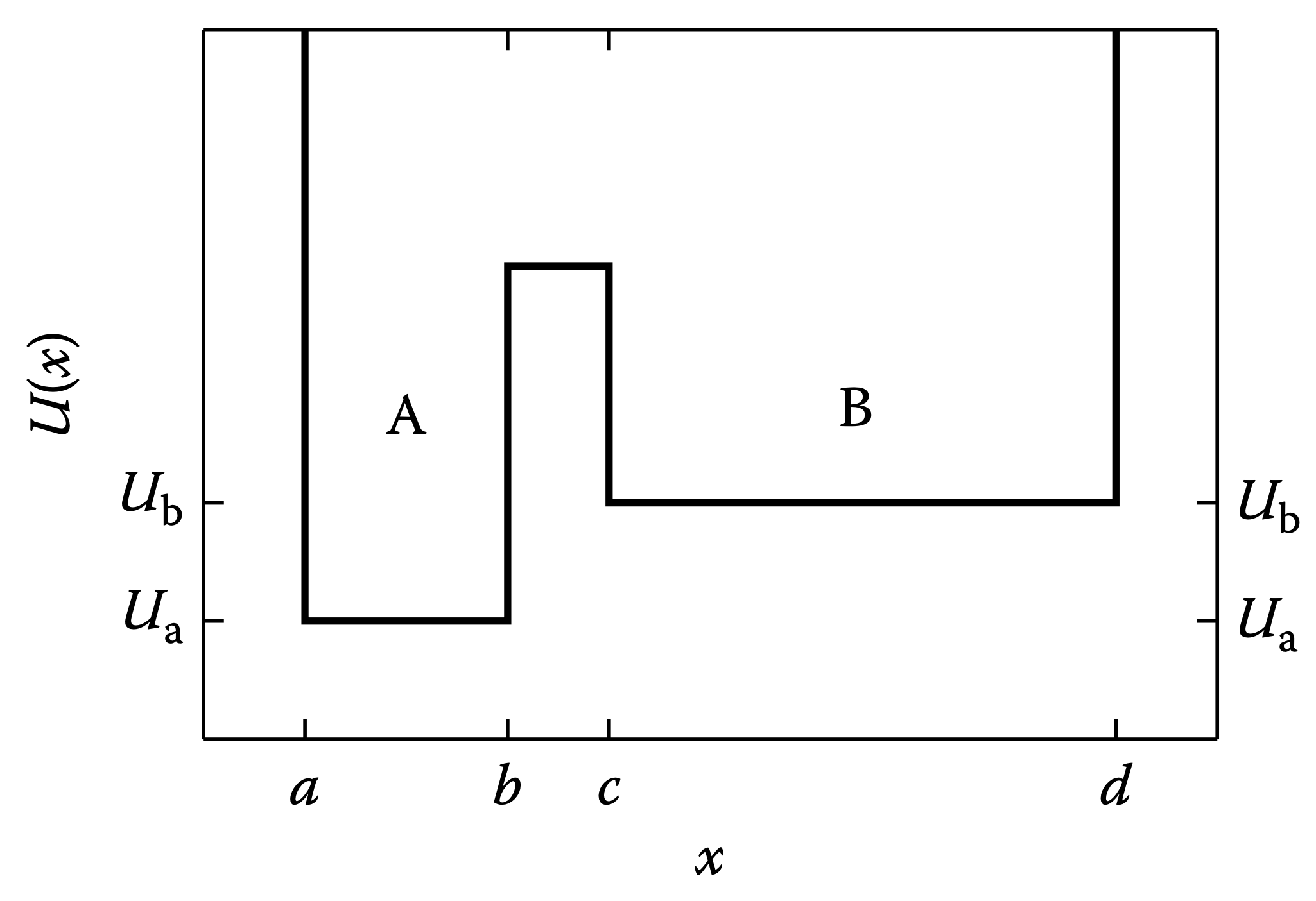
For each state, $A$ and $B$, what is $Z$, $F$, and $S$? Between the states, what is $\Delta F$ and $\Delta S$?