Mechanics 102

9/9/2025

print view

%%html
<script src="https://bits.csb.pitt.edu/preamble.js"></script>
<style>:root {--jp-cell-prompt-width: 0px; --jp-private-cell-scrolling-output-offset: 0px; --jp-code-padding: 0px; }</style>

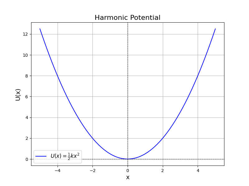
The Harmonic Oscillator

By Svjo - Previously uploaded version of Animated-mass-spring.gif here, CC BY-SA 3.0, Link

$$\Large U(x) = U_0 + \frac{1}{2} \kappa (x-x_0)^2$$

where $U_0$ is the baseline potential energy, $\kappa$ is the spring constant and $x_0$ is the center position.

%%capture
import numpy as np
import matplotlib.pyplot as plt

# Define the spring constant and the harmonic potential
k = 1  # Spring constant
def harmonic_potential(x):
    return 0.5 * k * x**2

# Define the range of x values
x = np.linspace(-5, 5, 500)

# Calculate the potential
U = harmonic_potential(x)

# Plot the harmonic potential
fig = plt.figure(figsize=(8, 6))
plt.plot(x, U, label=r'$U(x) = \frac{1}{2}kx^2$', color='blue')
plt.axhline(0, color='black', linewidth=0.8, linestyle='--')
plt.axvline(0, color='black', linewidth=0.8, linestyle='--')
plt.title('Harmonic Potential', fontsize=16)
plt.xlabel('x', fontsize=14)
plt.ylabel('U(x)', fontsize=14)
plt.legend(fontsize=12)
plt.grid(True);
fig.savefig('imgs/harmonic_potential.png')

%%html
<div id="sprintk" style="width: 500px"></div>
<script>
    var divid = '#sprintk';
	jQuery(divid).asker({
	    id: divid,
	    question: "What happens to the potential well as you increase the spring constant k?",
		answers: ["Gets narrower","Gets wider",'Moves up',"Moves down"],
        server: "https://bits.csb.pitt.edu/asker.js/example/asker.cgi",
		charter: chartmaker})
    
$(".jp-InputArea .o:contains(html)").closest('.jp-InputArea').hide();


</script>

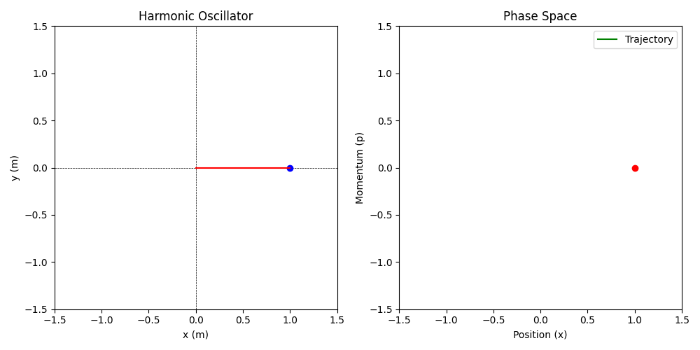
Configuration vs Phase Space

%%html
<div id="phasedim" style="width: 500px"></div>
<script>
    var divid = '#phasedim';
	jQuery(divid).asker({
	    id: divid,
	    question: "How many dimensions does the phase space of a molecule with N atoms have?",
		answers: ["2N","3N","6N","N^3",'2N^3'],
        server: "https://bits.csb.pitt.edu/asker.js/example/asker.cgi",
		charter: chartmaker})
    
$(".jp-InputArea .o:contains(html)").closest('.jp-InputArea').hide();


</script>

Newtonian

$$\Large F = - \frac{\partial U(x)}{\partial x} = - \frac{\partial}{\partial x} \left( U_0 + \frac{1}{2}kx^2 \right) = -kx$$ $$\Large F = ma = \frac{dp}{dt} = \frac{d}{dt} mv = \frac{d}{dt} m \frac{dx}{dt} = m\frac{d^2x}{dt^2}$$

$$\Large m\frac{d^2x}{dt^2} = -kx$$ This is the equation of motion for an object attached to a spring. The solution to this second order differential equation tells us how the system evolves.

Hamiltonian

$$\Large H = \mathrm{KE} + U = \frac{1}{2}\frac{p^2}{m} + \frac{1}{2}kx^2$$

$$\frac{dp}{dt} = - \frac{\partial H}{\partial x} = - \frac{\partial \left( \frac{1}{2}\frac{p^2}{m} + \frac{1}{2}kx^2\right)} {\partial x} = -kx $$ $$\frac{dx}{dt} = \frac{\partial H}{\partial p} = \frac{\partial \left( \frac{1}{2}\frac{p^2}{m} + \frac{1}{2}kx^2\right)} {\partial p} = \frac{p}{m}$$

We have a system of first order differential equations that tell us how the system evolves. If we solve for $\frac{dp}{dt}$ and substitute, we get our second order equations of motion.

Solution

What function satisfies this relationship?

$$m\frac{d^2x}{dt^2} = -kx$$

$$x(t) = A\cos(\omega t) + B \sin(\omega t)$$ where $$\omega = \sqrt{\frac{k}{m}} \\ A = x(0) \\ B = w^{-1}\frac{dx(0)}{dt}$$

mass = 1.0; k = 1.0   
omega = np.sqrt(k / mass) 
x0 = 1.0  # Initial position 
v0 = 0  # Initial velocity 

# Time settings
time_step = 0.02  # Time step (s)
total_time = 20.0  # Total simulation time (s)
times = np.arange(0, total_time, time_step)

# Solve the equations of motion
positions = x0 * np.cos(omega * times) + (v0 / omega) * np.sin(omega * times)
velocities = -x0 * omega * np.sin(omega * times) + v0 * np.cos(omega * times)

plt.figure(figsize=(10,4))
plt.plot(times,positions,label='$x(t)$')
plt.plot(times,velocities,label='$v(t)$')
plt.legend(); plt.xlabel('t');

%%html
<div id="harmmicro" style="width: 500px"></div>
<script>
    var divid = '#harmmicro';
	jQuery(divid).asker({
	    id: divid,
	    question: "What can be said about the probabilities of the microstates (positions in phase space) of this system?",
		answers: ["They are equal","Equal excluding extrema","Variable"],
        server: "https://bits.csb.pitt.edu/asker.js/example/asker.cgi",
		charter: chartmaker})
    
$(".jp-InputArea .o:contains(html)").closest('.jp-InputArea').hide();


</script>

Let's heat things up!

Boltzmann Distribution

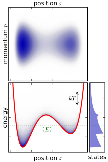
The Boltzmann distribution converts the energy landscape of a system into a probability distribution

$$\Large \rho(x) \propto e^{\frac{-E(x)}{k_B T}}$$

$k_B= 1.4\times 10^{-23} \,\mathrm{J\,K}^{-1}$ is Boltzmann constant

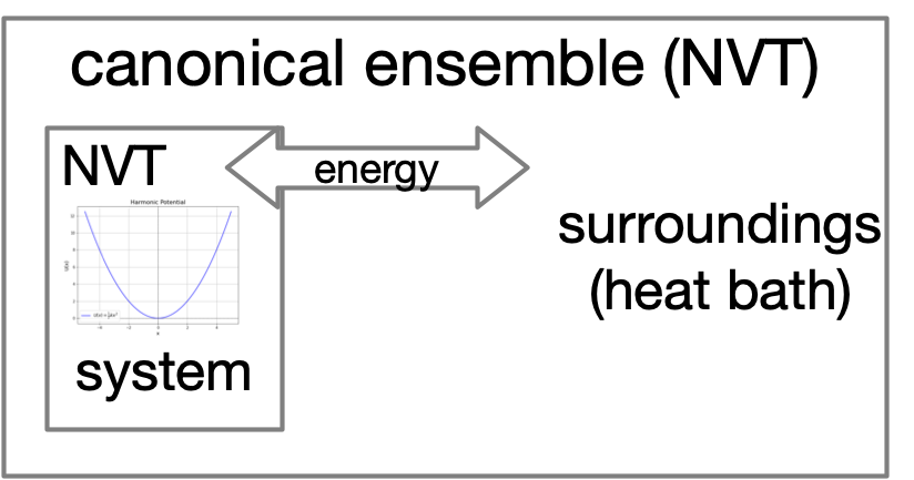
	microcanonical (NVE)	canonical (NVT)

%%html
<div id="boltz1" style="width: 500px"></div>
<script>
    var divid = '#boltz1';
	jQuery(divid).asker({
	    id: divid,
	    question: "Higher energy microstates are",
		answers: ["More probable","Less Probable","Depends"],
        server: "https://bits.csb.pitt.edu/asker.js/example/asker.cgi",
		charter: chartmaker})
    
$(".jp-InputArea .o:contains(html)").closest('.jp-InputArea').hide();


</script>

%%html
<div id="boltz2" style="width: 500px"></div>
<script>
    var divid = '#boltz2';
	jQuery(divid).asker({
	    id: divid,
	    question: "As temperature increases, higher energy microstates will become",
		answers: ["More probable","Less Probable","Depends"],
        server: "https://bits.csb.pitt.edu/asker.js/example/asker.cgi",
		charter: chartmaker})
    
$(".jp-InputArea .o:contains(html)").closest('.jp-InputArea').hide();


</script>

%%html
<div id="boltzneednorm" style="width: 500px"></div>
<script>
    var divid = '#boltzneednorm';
	jQuery(divid).asker({
	    id: divid,
	    question: "E(x) = 1/β.  What is the probability of x?",
		answers: ["1","e","β^2","1/e","None of the above"],
        server: "https://bits.csb.pitt.edu/asker.js/example/asker.cgi",
		charter: chartmaker})
    
$(".jp-InputArea .o:contains(html)").closest('.jp-InputArea').hide();


</script>

Partition Function

The normalization factor for the Boltzmann distribution is called the Partition Function

$$\Large \rho(x)= \frac{ e^{-E(x)/k_B T} }{\int_V \,e^{-E(x)/k_B T}dx} = \frac{ e^{-E(x)/k_B T} }{Z}$$

$$ \int_V \rho(x) = 1$$

$$\Large \hat{Z}\equiv \int_V \,e^{-U(x)/k_B T} dx = \lambda Z$$

Ensemble Properties

We can compute mean of any property of states (defined by function $g$) using the defition of expectation.

$$\Large \langle g \rangle = \int_V \,g(x)\,\rho(x) dx \\ \Large \langle g \rangle = \frac{\int_V g(x)\, e^{-U(x)/k_B T}dx}{\hat{Z}} $$

Average Energy of Harmonic System

$$\Large U_{\mathrm{harm}}= U_0 + \left( \frac{\kappa}{2}\right)(x-x_0)^2 $$

$$\Large \langle U_{\mathrm{harm}} \rangle = \frac{\int_V U_{\mathrm{harm}}(x)\, e^{-U_{\mathrm{harm}}(x)/k_B T}dx} {\int_V e^{-U_{\mathrm{harm}}(x)/k_B T}dx}$$

What is $\hat{Z}$?

Partition Function of Harmonic Potential

$$\Large \hat{Z}_{\mathrm{harm}}= \int_V e^{-\left ( U_0 + \left( \frac{\kappa}{2}\right)(x-x_0)^2 \right)/k_B T}dx \\ \Large \hat{Z}_{\mathrm{harm}}= e^{-U_0/k_B T}\int_{-\infty}^{\infty} e^{-\frac{\kappa (x-x_0)^2}{2k_B T}}dx = e^{-U_0/k_B T}\sqrt{\frac{2\pi k_B T}{\kappa}}$$

Average Energy

$$\Large \langle U_{\mathrm{harm}} \rangle = \frac{\int_V U_{\mathrm{harm}}(x)\, e^{-U_{\mathrm{harm}}(x)/k_B T}dx} {\int_V e^{-U_{\mathrm{harm}}(x)/k_B T}dx}$$

This can be solved exactly (using additional integration identities) $$\Large \langle U_{\mathrm{harm}}\rangle= U_0 + \frac{1}{2}k_BT$$

This is the equipartition theorem. Any coordinate whose energy depends quadratically on its value (e.g., velocity $= \frac{mv^2}{2}$) will have an average energy of $\frac{1}{2}k_BT$.

Notice there is no $\kappa$ in this result!

Each degree of freedom that appears quadratically in the expression for the total energy contributes an average energy of $\frac{1}{2}k_BT$ to the system

%%html
<div id="equipartatom" style="width: 500px"></div>
<script>
    var divid = '#equipartatom';
	jQuery(divid).asker({
	    id: divid,
	    question: "What is the average kinetic energy of a single atom (NVT)?",
		answers: ["½kᵦT","kᵦT","³⁄₂kᵦT","-kᵦT"],
        server: "https://bits.csb.pitt.edu/asker.js/example/asker.cgi",
		charter: chartmaker})
    
$(".jp-InputArea .o:contains(html)").closest('.jp-InputArea').hide();


</script>

The Full (1D) Partition Function

$$\Large \frac{m}{h} \int_{-\infty}^{\infty} \int_{-\infty}^{\infty} e^{-\frac{\frac{mv^2}{2} + U(x)}{k_B T}} dx dv$$

$$= \Large \frac{m}{h} \int_{-\infty}^{\infty} e^{-\frac{\frac{mv^2}{2} }{k_B T}} dv \int_{-\infty}^{\infty} e^{-\frac{U(x)}{k_B T}} dx$$

$$ = \Large \frac{m}{h} \sqrt{\frac{2\pi k_B T}{m}} \int_{-\infty}^{\infty} e^{-\frac{U(x)}{k_B T}} dx$$

$$ = \Large \frac{1}{\lambda} \hat{Z}$$

States

Biomolecules have an essentially infinite set of configurations. We are interested in the sets of configurations that behave in a “similar way.” States represent a way to cluster configurations of biomolecules by function.

• What are the relative probabilities to observe molecule in state A vs. state B?
• What properties affect these probabilities?

State Probabilties

$$ p_A = \hat{Z}^{-1}\int_{V_A} e^{-U(x)/k_B T} dx \approx \hat{Z}^{-1}\int_{-\infty}^{\infty} e^{-U_A(x)/k_B T} dx \\ p_B = \hat{Z}^{-1}\int_{V_B} e^{-U(x)/k_B T dx} \approx \hat{Z}^{-1}\int_{-\infty}^{\infty} e^{-U_B(x)/k_B T dx}$$

The ratio of probabilties is given by:

$$\Large \frac{p_A}{p_B} = \frac{\int_{V_A} e^{-U(x)/k_B T}dx} {\int_{V_B} e^{-U(x)/k_B T} dx} \approx \sqrt{\frac{\kappa_b}{\kappa_a}}$$

%%html
<div id="harmstate1" style="width: 500px"></div>
<script>
    var divid = '#harmstate1';
	jQuery(divid).asker({
	    id: divid,
	    question: "In this diagram, which state is more probable?",
		answers: ["A","B","Neither"],
        server: "https://bits.csb.pitt.edu/asker.js/example/asker.cgi",
		charter: chartmaker})
    
$(".jp-InputArea .o:contains(html)").closest('.jp-InputArea').hide();


</script>

Free Energy of a State

$$\Large \frac{p_A}{p_B} = \frac{\int_{V_A} e^{-U(x)/k_B T}\,dx} {\int_{V_B} e^{-U(x)/k_B T}\,dx} \equiv \frac{e^{-F_A/k_B T}} {e^{-F_B/k_B T}}$$

In general for a state $i$ we have

$$\Large F_i = -k_B T \ln \left( {{Z_i}}\right)$$

This is we call the free energy of state $i$.

The probability distribution of states follows the Boltzmann distribution in free energy $\Large p_i \propto e^{-F_i/k_BT}$

Free Energy of Harmonic Well

$$\Large U(x)= U_0 + \left( \frac{\kappa}{2}\right)(x-x_0)^2$$

$$\Large \hat{Z}_i =\int_{V} e^{-U_0/k_BT - \frac{1}{2}\kappa_i(x-x_0)^2/k_B T}dx = e^{-U_0/k_BT}\sqrt{\frac{2\pi k_B T}{\kappa}}$$ $$\Large F = U_0 - k_B T \ln \left(\lambda^{-1}\sqrt{\frac{2\pi k_B T}{\kappa}}\right)$$

Entropy of Harmonic Well

$$\Large S\equiv \frac{\langle E\rangle - F}{T}$$ $$ S = \frac{ \color{blue}{ \langle K\rangle } + \color{purple}{\langle U\rangle} - \color{green}{F}}{T}= \frac{\color{blue}{\frac{k_BT}{2}} + \color{purple}{U_0 + \frac{k_BT}{2}} - \color{green}{\left( U_0 - k_B T \ln \left(\lambda^{-1}\sqrt{\frac{2\pi k_B T}{\kappa_i}}\right)\right)}}{T} $$

$$\Large S = k_B + k_B \ln \left( \lambda^{-1}{\sqrt{\frac{2 \pi k_B T}{\kappa}}} \right) $$

%%html
<div id="widthentropy" style="width: 500px"></div>
<script>
    var divid = '#widthentropy';
	jQuery(divid).asker({
	    id: divid,
	    question: "In this diagram, which state has higher entropy?",
		answers: ["A","B","Neither"],
        server: "https://bits.csb.pitt.edu/asker.js/example/asker.cgi",
		charter: chartmaker})
    
$(".jp-InputArea .o:contains(html)").closest('.jp-InputArea').hide();


</script>

Entropy

Alternatively: $$\Large F = \langle E \rangle - TS$$

The probability of a state $i$ can then be written $$\Large p_i \propto e^{-F_i/k_B T}= e^{+S_i/k_B} e^{-\langle E\rangle_i /k_B T}$$

The Boltzmann factor for a state is just the Boltzmann factor for its average energy times a factor, which will turn out to be related to volume in configuration space (or number of states in a discrete space).

Entropy

$$\Large S = k_B \ln \Omega$$

(Only applies to microcanonical ensemble.)

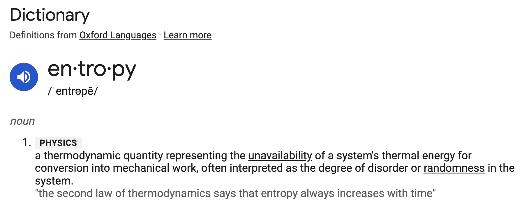
Gibb's Entropy

$$S_{\large \mathrm{Gibbs}}= -k_B\sum_i p_i \ln p_i$$

What happens when $p_i = \frac{1}{N}$?

What about $p_i = Z^{-1} e^{-\frac{U(i)}{k_B T}}$ ?

Shannon Entropy (Information Theory)

$$\Large S_{\mathrm{Shannon}}= -\sum_i p_i \log_2 p_i$$

With $\log_2$ the units of Shannon entropy are "bits" or "Shannons."

In information theory, the entropy of a random variable quantifies the average level of uncertainty or information associated with the variable's potential states or possible outcomes. This measures the expected amount of information needed to describe the state of the variable, considering the distribution of probabilities across all potential states.

--Wikipedia)

%%html
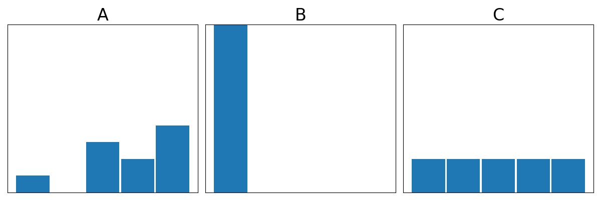
<div id="distdisorder" style="width: 500px"></div>
<script>
    var divid = '#distdisorder';
	jQuery(divid).asker({
	    id: divid,
	    question: "Which distribution is most disordered (highest entropy)?",
		answers: ["A","B","C"],
        server: "https://bits.csb.pitt.edu/asker.js/example/asker.cgi",
		charter: chartmaker})
    
$(".jp-InputArea .o:contains(html)").closest('.jp-InputArea').hide();


</script>

Summary

	Microstate = single configuration	Macrostate = set of configurations
Partition function	-	$ \hat{Z}= \int_V e^{-U(x)/k_BT} dx$
Configuration energy	$U(x)$	$\langle U \rangle = \hat{Z}^{-1} \int_V U(x)\,e^{-U(x)/k_B T} dx$
Relative probability	$e^{-U(x)/k_B T}$	$e^{-F/k_B T} \propto e^{S/k_B}\,e^{-\langle U \rangle/k_B T}$
Free energy	-	$F = - k_B T \ln Z$
Entropy	-	$S = \frac{k_B}{2} + \frac{\langle U\rangle-F}{T} $

Double square well potential

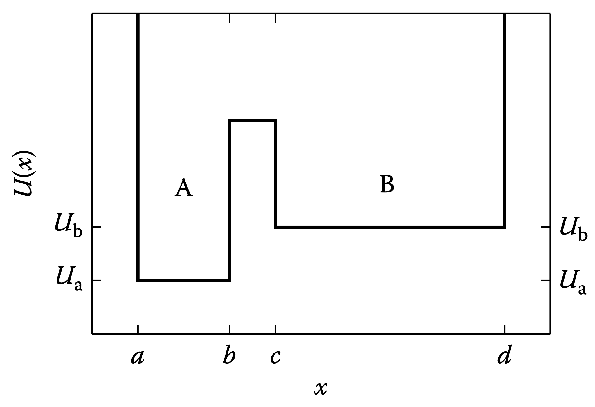
For each state, $A$ and $B$, what is $Z$, $F$, and $S$? Between the states, what is $\Delta F$ and $\Delta S$?