%%html
<script src="https://bits.csb.pitt.edu/preamble.js"></script>
<style>:root {--jp-cell-prompt-width: 32px}</style>
Reminders
| Microstate = single configuration | Macrostate = set of configurations | |
|---|---|---|
| Partition function | - | $ \hat{Z}= \int_V e^{-U(x)/k_BT} dx$ |
| Configuration energy | $U(x)$ | $\langle U \rangle = \hat{Z}^{-1} \int_V U(x)\,e^{-U(x)/k_B T} dx$ |
| Unnormalized probability | $e^{-U(x)/k_B T}$ | $e^{-F/k_B T} \propto e^{S/k_B}\,e^{-\langle U \rangle/k_B T}$ |
| Free energy | - | $F = - k_B T \ln Z$ |
| Entropy | - | $S = \frac{\langle U\rangle-F}{T} $ |
$$\Large \Delta F = \Delta U - T \Delta S$$
Here $U \equiv \langle E \rangle $, the average energy.
$S$ is the entropy, which is related to the number of states and their probabilities - how disordered the system is.
Double square well potential
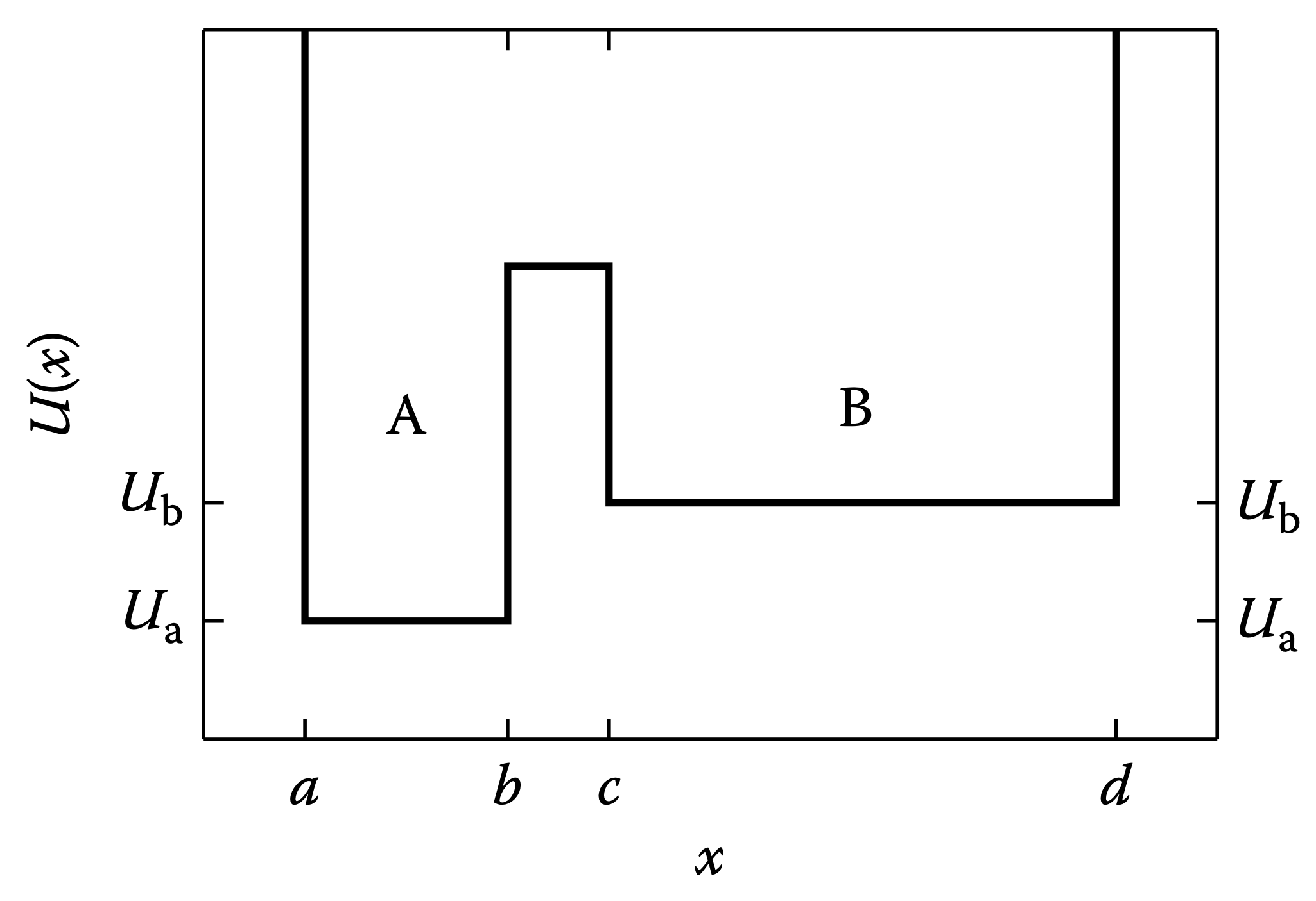
For each state, $A$ and $B$, what is $Z$, $F$, and $S$? Between the states, what is $\Delta F$ and $\Delta S$?
Multidimensional Statistical Mechanics
One "atom" in two dimensions
For $U(x,y) = 0$
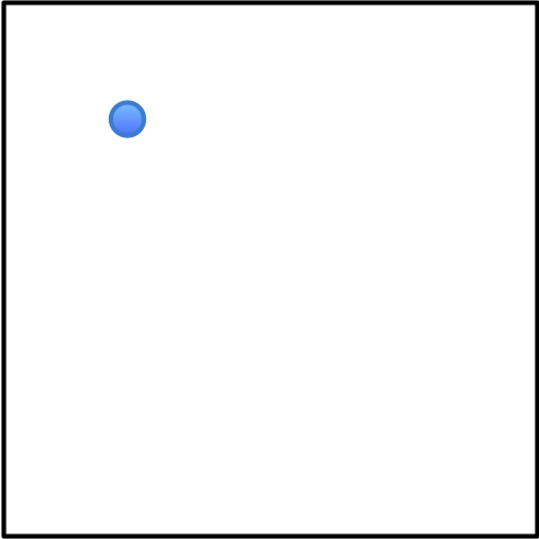
$$\langle U \rangle = 0$$
$$\langle KE \rangle = k_BT$$
$$S = \frac{\langle E \rangle - F}{T} = \frac{k_BT - (-k_BT \ln Z)}{T} = k_B \left( 1 + \ln \left( \frac{L}{\lambda} \right)^2 \right)$$
$$\Large S \approx k_B \ln \left( \frac{L}{\lambda} \right)^2 $$
Two particles
Particles are still non-interacting: $U(x^A, y^A, x^B, y^B) = 0$.
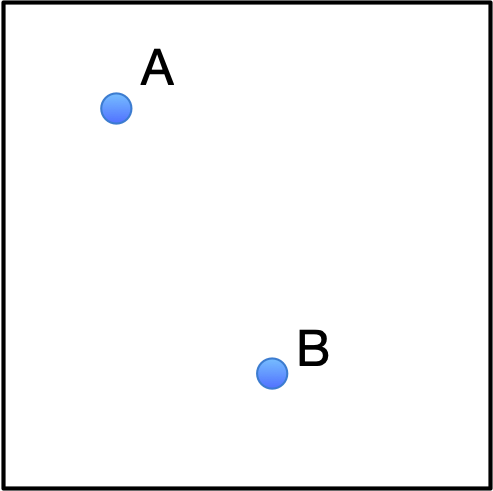
$$ \begin{align*} Z &= \left( \frac{1}{h} \int_{-\infty}^{+\infty} dp_x^A e^{-\left[(p_x^A)^2 / 2m_A\right] / k_B T} \right) \left( \frac{1}{h} \int_{-\infty}^{+\infty} dp_y^A e^{-\left[(p_y^A)^2 / 2m_A\right] / k_B T} \right) \\ &\quad \times \left( \frac{1}{h} \int_{-\infty}^{+\infty} dp_x^B e^{-\left[(p_x^B)^2 / 2m_B\right] / k_B T} \right) \left( \frac{1}{h} \int_{-\infty}^{+\infty} dp_y^B e^{-\left[(p_y^B)^2 / 2m_B\right] / k_B T} \right) \\ &\quad \times \int_0^L dx^A \int_0^L dy^A \int_0^L dx^B \int_0^L dy^B \exp\left[-\frac{U(x^A, y^A, x^B, y^B)}{k_B T}\right] \\ &= \frac{L^4}{\lambda_A^2 \lambda_B^2}. \end{align*} $$
$$\Large S \approx k_B \ln \frac{L^4}{\lambda_A^2 \lambda_B^2} = k_B \left[ \ln \left( \frac{L}{\lambda_A} \right)^2 + \ln \left( \frac{L}{\lambda_B} \right)^2 \right]$$
Diatomic "molecule" in 2D
Assume the two particles are connected by a spring with constant $\kappa$ so that the potential energy in terms of the distances between them, $r$, is $$U = \frac{1}{2}\kappa (r - r_0)^2, \mathrm{where}\,\, r = \sqrt{(x^A-x^B)^2 + (y^A-y^B)^2}$$
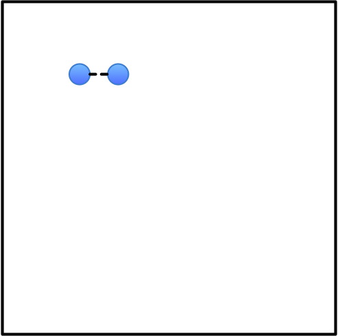
$$ Z = \frac{1}{\lambda_A^2 \lambda_B^2} \int_0^L dx^A \int_0^L dy^A \int_0^L dx^B \int_0^L dy^B \, e^{-U(r)/k_B T}$$
Convert to polar coordinates for B relative to A.
$$\int \int \int \int dx^A dy^A dx^B dy^B = \int \int \int \int dx^A dy^A r \, dr \, d\phi$$
Change variables to describe the molecule
The potential depends only on the distance between the atoms,
$$ U = U(r) $$
so it is more useful to describe the system using:
- the position of atom A: $(x_A,y_A)$
- the displacement of B relative to A: $(\Delta x,\Delta y)$
where
$$ \Delta x=x_B-x_A,\qquad \Delta y=y_B-y_A $$
The volume element is unchanged:
$$ dx_A\,dy_A\,dx_B\,dy_B = dx_A\,dy_A\,d\Delta x\,d\Delta y $$
Now use polar coordinates for the relative displacement:
$$ \Delta x=r\cos\phi,\qquad \Delta y=r\sin\phi, $$
and
$$ d\Delta x\,d\Delta y = \left|\det J_F(r,\phi)\right|\,dr\,d\phi = r\,dr\,d\phi. $$
Change of Variables
In vector calculus, the Jacobian matrix of a vector-valued function of several variables is the matrix of all its first-order partial derivatives. The Jacobian can be understood by considering a unit area in the new coordinate space; and examining how that unit area transforms when mapped into xy coordinate space in which the integral is visually understood. --Wikipedia
$$\mathbf{f} : \mathbf{R}^n → {R}^m$$
$$\mathbf{J_f} = \begin{bmatrix} \dfrac{\partial \mathbf{f}}{\partial x_1} & \cdots & \dfrac{\partial \mathbf{f}}{\partial x_n} \end{bmatrix} = \begin{bmatrix} \nabla^{\mathsf{T}} f_1 \\ \vdots \\ \nabla^{\mathsf{T}} f_m \end{bmatrix} = \begin{bmatrix} \dfrac{\partial f_1}{\partial x_1} & \cdots & \dfrac{\partial f_1}{\partial x_n}\\ \vdots & \ddots & \vdots\\ \dfrac{\partial f_m}{\partial x_1} & \cdots & \dfrac{\partial f_m}{\partial x_n} \end{bmatrix}$$
Cartesian to Polar
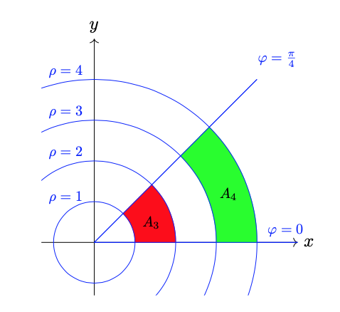
$$ \Large {\mathbf F}(r,\phi) = \begin{pmatrix} \Delta x \\ \Delta y \end{pmatrix} = \begin{pmatrix} r\cos\phi \\ r\sin\phi \end{pmatrix} $$
$$\Large \mathbf J_{\mathbf F}(r, \phi) = \begin{bmatrix} \frac{\partial x}{\partial r} & \frac{\partial x}{\partial\phi}\\[0.5ex] \frac{\partial y}{\partial r} & \frac{\partial y}{\partial\phi} \end{bmatrix} = \begin{bmatrix} \cos\phi & - r\sin \phi \\ \sin\phi & r\cos \phi \end{bmatrix}$$
What is the determinant of $\mathbf J_{\mathbf F}$?
Change of Variables
$$ \iint_{A_{\Delta x,\Delta y}} f(\Delta x,\Delta y)\,d\Delta x\,d\Delta y = \iint_{A_{r,\varphi}} f(r\cos\varphi,r\sin\varphi)\, \left|\det J_F(r,\varphi)\right|\, dr\,d\varphi $$
For polar coordinates,
$$ \left|\det J_F(r,\varphi)\right|=r, $$
so
$$ \iint_{A_{\Delta x,\Delta y}} f(\Delta x,\Delta y)\,d\Delta x\,d\Delta y = \iint_{A_{r,\varphi}} f(r\cos\varphi,r\sin\varphi)\, r\,dr\,d\varphi. $$
Diatomic "molecule" in 2D
$$ Z = \frac{1}{\lambda_A^2 \lambda_B^2} \int_0^L dx^A \int_0^L dy^A \int_0^{r_{\text{max}}} r \, dr \int_0^{2\pi} d\phi \, e^{-U(r)/k_B T}$$
$$ \simeq \frac{2\pi}{\lambda_A^2 \lambda_B^2} \int_0^L dx^A \int_0^L dy^A \int_0^{r_{\text{max}}} dr \, r \, e^{-\frac{\kappa(r - r_0)^2}{2k_B T}}$$
$$ \simeq \frac{2\pi L^2}{\lambda_A^2 \lambda_B^2} \int_0^{\infty} dr \, r e^{-\frac{\kappa(r - r_0)^2}{2k_B T}} \simeq \frac{2\pi L^2}{\lambda_A^2 \lambda_B^2} r_0 \int_0^{\infty} dr \, e^{-\frac{\kappa(r - r_0)^2}{2k_B T}}$$
$$\Large \simeq \frac{2\pi L^2}{\lambda_A^2 \lambda_B^2} r_0 \sqrt{\frac{2\pi k_B T}{\kappa}} $$
$$S \simeq k_B \ln Z = k_B \left[ \ln \left( \frac{L^2}{\lambda_A^2} \right) + \ln \left( \frac{ 2\pi r_0 \sqrt{2\pi k_B T / \kappa}}{\lambda_B^2} \right) \right]$$
Comparing Entropies
$$\Large S_\mathrm{one\ atom} \approx k_B \ln \left( \frac{L^2}{\lambda^2} \right) $$
$$\Large S_{\mathrm{two\ atom}} \approx k_B \ln \frac{L^4}{\lambda_A^2 \lambda_B^2} = k_B \left[ \ln \left( \frac{L^2}{\lambda_A^2} \right) + \ln \left( \frac{L^2}{\lambda_B^2} \right) \right]$$
$$\Large S_{\mathrm{diatomic}} \simeq k_B \ln Z = k_B \left[ \ln \left( \frac{L^2}{\lambda_A^2} \right) + \ln \left( \frac{r_0 \sqrt{2\pi k_B T / \kappa}}{\lambda_B^2} \right) \right]$$
The General Unimolecular Partition Function
$$\Large Z = \frac{1}{\mathcal{N}_D} \left[ \prod_{i=1}^N \lambda_i^{-3} \right] \int dx_1 \, dy_1 \, dz_1 \, \dots \, dx_N \, dy_N \, dz_N \, e^{-U(\mathbf{r}^N)/k_B T} $$
$$\Large = \frac{1}{\mathcal{N}_D} \left[ \prod_{i=1}^N \lambda_i^{-3} \right] \int d\mathbf{r}^N \, e^{-U(\mathbf{r}^N)/k_B T}$$
where $\mathcal{N}_D$ is the degeneracy number that prevents overcounting of of indistinguishable states and $\mathbf{r}^N$ is the position vector $(x_1,y_1,z_1,\cdots,x_N,y_N,z_N$).
Problem: For any useful energy potential, $U(\mathbf{r}^N)$ cannot be factored into separable components and this integral has no closed form solution.
%%html
<div id="gridZ" style="width: 500px"></div>
<script>
    var divid = '#gridZ';
	jQuery(divid).asker({
	    id: divid,
	    question: "Suppose we want to numerically integrate the general unimolecular partition function for a molecule with $N$ atoms using a cubic grid with side lengths 100Å and a 0.1Å resolution.  How many energy evaluations do I need to perform?",
		answers: ["3000N","N^1000","1000^(3N)","10^(3N)"],
        server: "https://bits.csb.pitt.edu/asker.js/example/asker.cgi",
		charter: chartmaker})

$(".jp-InputArea .o:contains(html)").closest('.jp-InputArea').hide();


</script>
%%html
<div id="gridZ2" style="width: 500px"></div>
<script>
    var divid = '#gridZ2';
	jQuery(divid).asker({
	    id: divid,
	    question: "What will be the most common value inside the integral?",
		answers: ["0","1","e","unknown"],
        server: "https://bits.csb.pitt.edu/asker.js/example/asker.cgi",
		charter: chartmaker})

$(".jp-InputArea .o:contains(html)").closest('.jp-InputArea').hide();


</script>
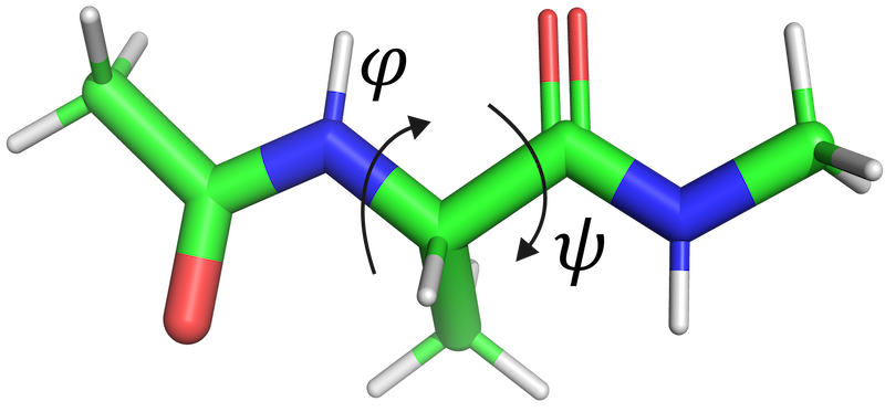
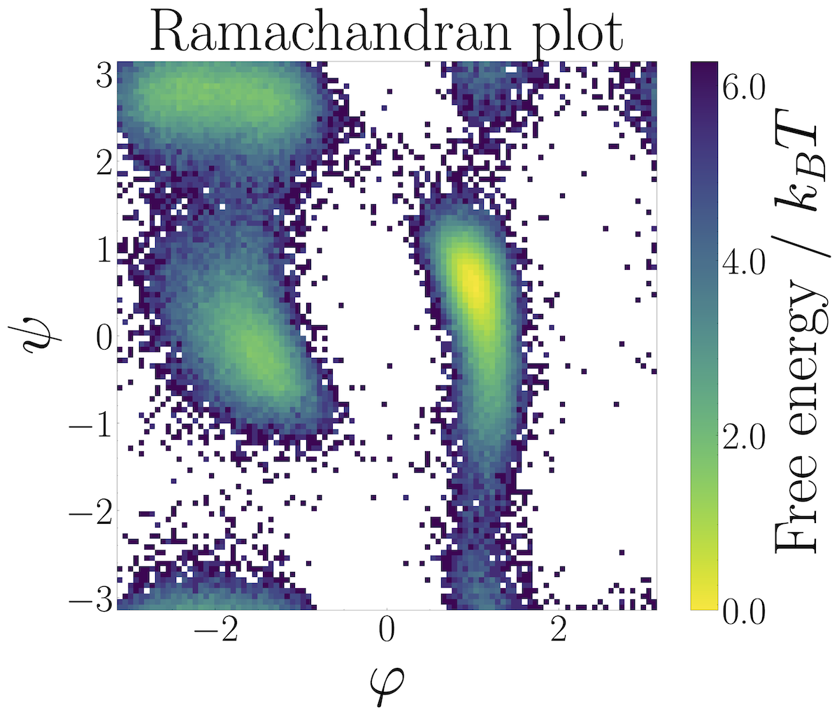
Alanine Dipeptide Free Energy Surface
Recall: Newton's Equations of Motion
$$\Large F = ma = \frac{dp}{dt} = \frac{d}{dt} mv = \frac{d}{dt} m \frac{dx}{dt} = m\frac{d^2x}{dt^2}$$

For harmonic oscillator:
$$m\frac{d^2x}{dt^2} = -\kappa x$$
$$x(t) = A\cos(\omega t) + B \sin(\omega t)$$ where $$\omega = \sqrt{\frac{\kappa}{m}} \\ A = x(0) \\ B = \omega^{-1}\frac{dx(0)}{dt}$$
import numpy as np
import matplotlib.pyplot as plt
from matplotlib.animation import FuncAnimation, PillowWriter
from matplotlib.gridspec import GridSpec
%%html
<div id="whatens" style="width: 500px"></div>
<script>
    var divid = '#whatens';
	jQuery(divid).asker({
	    id: divid,
	    question: "What ensemble are we simulating?",
		answers: ["NVT","NVE","NPT","String"],
        server: "https://bits.csb.pitt.edu/asker.js/example/asker.cgi",
		charter: chartmaker})

$(".jp-InputArea .o:contains(html)").closest('.jp-InputArea').hide();


</script>
Euler's Method

Any interesting system will not have an analytic solution, so we must integrate the equations of motions. Let's apply Euler's method to the Hamiltonian equations of motion:
$$\frac{dp}{dt} = - \frac{\partial H}{\partial x} = - \frac{\partial \left( \frac{1}{2}\frac{p^2}{m} + \frac{1}{2}kx^2\right)} {\partial x} = -kx $$ $$\frac{dx}{dt} = \frac{\partial H}{\partial p} = \frac{\partial \left( \frac{1}{2}\frac{p^2}{m} + \frac{1}{2}kx^2\right)} {\partial p} = \frac{p}{m}$$
Numerically integrate (switching to velocity from momentum so role of mass is obvious): $$\Large x_{n+1} = x_n + v_n \Delta t $$ $$\Large v_{n+1} = v_n - \frac{k}{m} x_n \Delta t$$
m = 1      # Mass
k = 1      # Spring constant
x_0 = 1    # Initial position
v_0 = 0    # Initial velocity
dt = 0.02

t = np.arange(0, 25, dt)

# Arrays to store position and velocity
x = np.zeros_like(t)
v = np.zeros_like(t)

# Initial conditions
x[0] = x_0
v[0] = v_0

# Euler's method loop
for i in range(len(t) - 1):
    x[i + 1] = x[i] + v[i] * dt
    v[i + 1] = v[i] - (k / m) * x[i] * dt


make_harmonic_anim(t, x,v,"imgs/spring_euler_hist.png");

Euler's method is problematic
$$\Large x_{n+1} = x_n + v_n \Delta t $$ $$\Large v_{n+1} = v_n - \frac{k}{m} x_n \Delta t$$
Does not conserve energy (technically speaking, it is neither time reversible nor symplectic).
energies = 0.5*k*x**2 + 0.5*m*v**2
print(f'Mean: {energies.mean()}  Std: {energies.std()}')
Mean: 0.6485564507647078 Std: 0.09339835794245747
%%html
<div id="whatshould" style="width: 500px"></div>
<script>
    var divid = '#whatshould';
	jQuery(divid).asker({
	    id: divid,
	    question: "What should the mean and std be?",
		answers: ["0,0","0.5,0.5","0.5,0","0,1"],
        server: "https://bits.csb.pitt.edu/asker.js/example/asker.cgi",
		charter: chartmaker})

$(".jp-InputArea .o:contains(html)").closest('.jp-InputArea').hide();


</script>
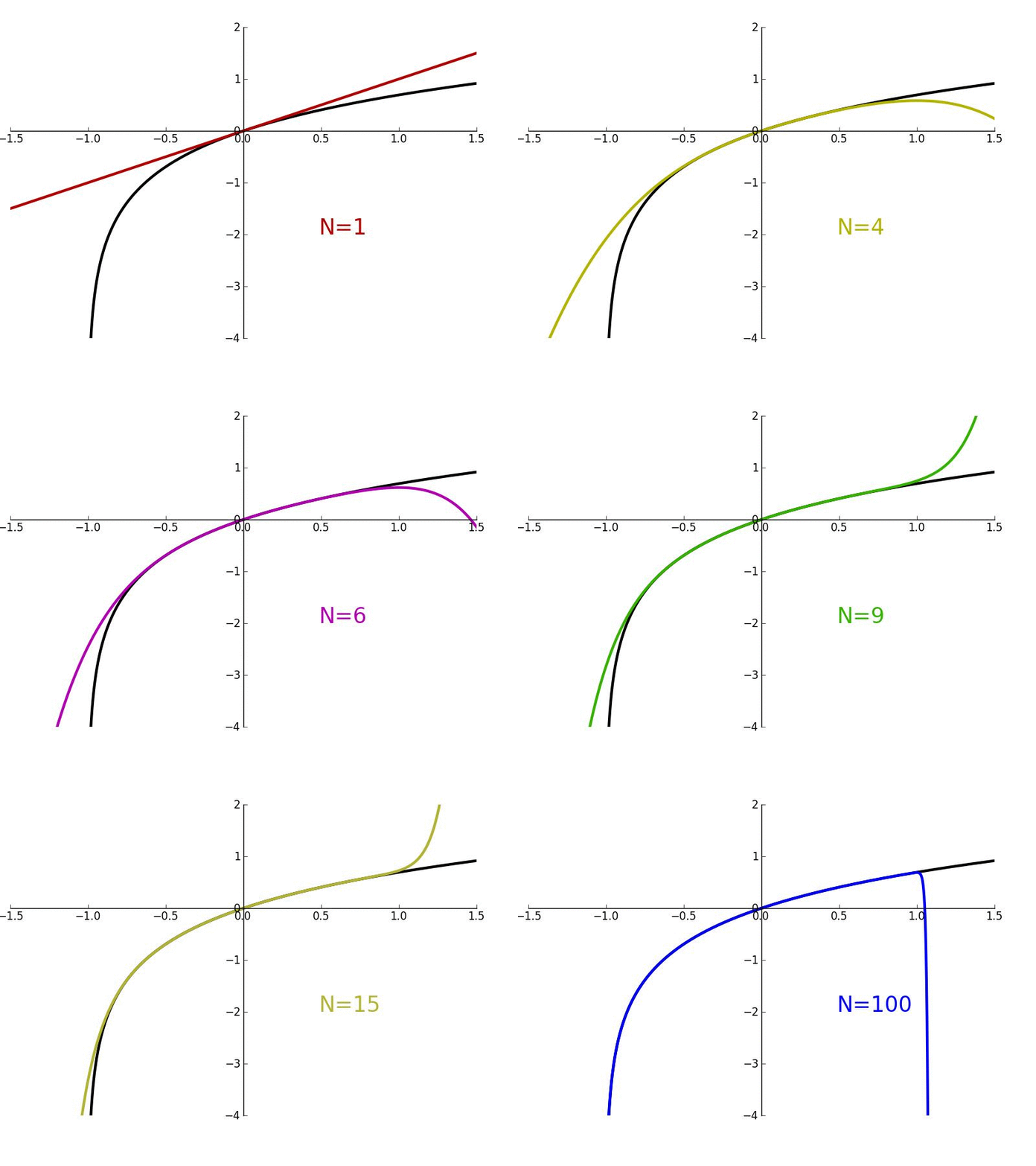
Mathematical Aside: Taylor Series
A way to approximate any differentiable function around a given point $a$ as a finite sum of polynomials: $$\Large f(x) \approx f(a) + \frac {f'(a)}{1!}(x-a) + \frac{f''(a)}{2!} (x-a)^2+ \cdots = \sum_{n=0} ^ {\infty} \frac {f^{(n)}(a)}{n!} (x-a)^{n}$$
Example: Approximating Bond Potential
Let's model the potential energy, $U$, of a covalent bond using a Lennard-Jones potential: $$U(r) = \frac{a}{r^{12}} - \frac{b}{r^6}$$ This is not a great approximation for covalent bonds, but it isn't the worst either and will be mathematically fun.
For a given well depth $U_0$ (minimum energy) and equilibrium position $r_0$ (bond length) determine the parameters $a$ and $b$ and then use this result to do a second order Taylor series expansion around $r_0$ to get a harmonic approximation, $H(r)$, of the potential energy.
Example: Approximating Bond Potential
$$U(r_0) = U_0 = \frac{a}{r_0^{12}} - \frac{b}{r_0^6}$$ $$U'(r_0) = 0 = \frac{-12a}{r_0^{13}} + \frac{6b}{r_0^7}$$
$$b = -2U_0 r_0^6$$ $$a = -U_0 r_0^{12}$$
Taylor Approximation
$$\Large U(r)_\text{approx} = U(r_0) + (r - r_0) U'(r_0) + \frac{(r - r_0)^2 U''(r_0)}{2} + \dots $$
$$U''(r_0) = \frac{156a}{r_0^{14}} - \frac{42b}{r_0^8} = \frac{-156U_0}{r_0^2} + \frac{84U_0}{r_0^2} = \frac{-72U_0}{r_0^2} $$
$$\Large U(r)_\text{approx} = U_0 + \frac{1}{2} K (r - r_0)^2 \quad \text{with} \quad K = \frac{-72U_0}{r_0^2}$$
r = np.linspace(.5,2.5,100)
U0 = -1
r0 = 1
a = -U0*r0**12
b = -2*U0*r0**6
K = -72*U0/r0**2
plt.plot(r,a/(r**12) - b/(r**6),label='LJ(r)')
plt.plot(r,U0+K*(r-r0)**2/2,label='H(r)')
plt.ylim(-1,0); plt.xlabel('r'); plt.ylabel('U(r)'); plt.legend();


Bond Oscillations
The frequency of oscillation $f$ is given by $$f = \frac{1}{2\pi}\sqrt{\frac{\kappa}{m}}$$ where $m$ is the mass and for two particles is the reduced mass: $$m=\frac{m_1m_2}{m_1+m_2}$$
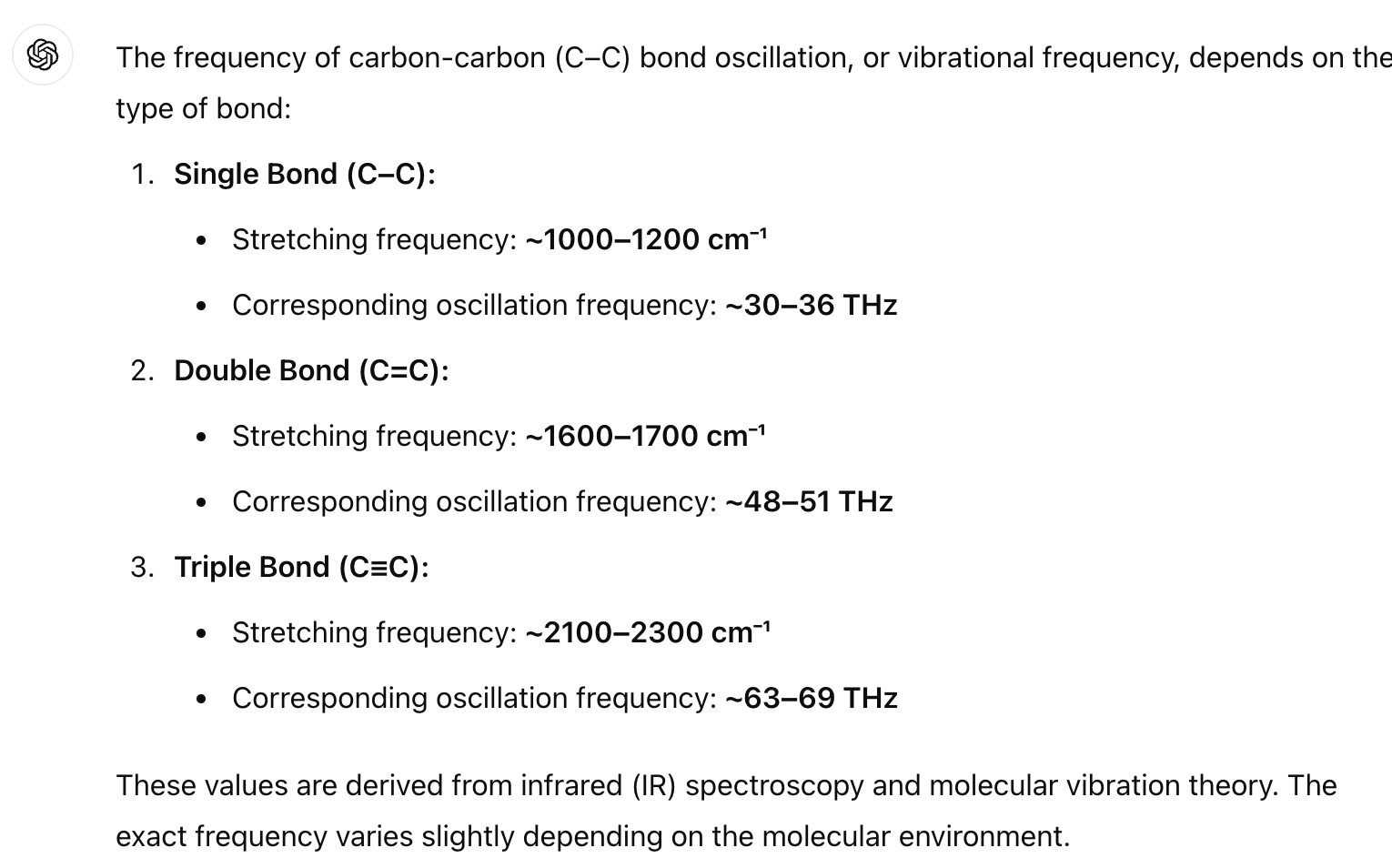
For a C-C bond assume C has a mass of 12 Daltons, the optimal bond length ($r_0$) is 150 picometers, and the bond energy ($U_0$) is -80 kcal/mol. What is the frequency in Hertz of this bond?
from openmm.unit import *
r0 = 150*picometer
U0 = -80*kilocalorie_per_mole
K = -72*U0/(r0)**2
m = (12*12)/(12+12)*dalton

f = sqrt(K/m)/(2*math.pi)
f
Quantity(value=67.245050959173, unit=/picosecond)
1/f.in_units_of(femtosecond**-1)
Quantity(value=14.870982856524824, unit=femtosecond)
f'{f.value_in_unit(seconds**-1):g}'
'6.72451e+13'
Back to dynamics... Verlet Integrator
Take the Taylor series of the positions around time $t$. $$\small f(x) \approx f(a) + \frac {f'(a)}{1!}(x-a) + \frac{f''(a)}{2!} (x-a)^2+ \cdots = \sum_{n=0} ^ {\infty} \frac {f^{(n)}(a)}{n!} (x-a)^{n}$$
$$ x(t+\Delta t) = x(t) + x'(t) \Delta t + \frac{x''(t)}{2} \Delta t^2+ \frac{x'''(t)}{6} \Delta t^3 + \mathcal{O}(\Delta t^4)$$
$$ x(t-\Delta t) = x(t) - x'(t) \Delta t + \frac{x''(t)}{2} \Delta t^2 - \frac{x'''(t)}{6} \Delta t^3 + \mathcal{O}(\Delta t^4)$$
adding these together we get
$$\Large x(t+\Delta t) + x(t-\Delta t) = 2x(t) + x''(t) \Delta t^2 + \mathcal{O}(\Delta t^4)$$
Harmonic Verlet
Solving for $x(t+\Delta t)$
$$\Large x(t+\Delta t) = 2x(t) - x(t-\Delta t) + x''(t) \Delta t^2 + \mathcal{O}(\Delta t^4)$$
Recall for a harmonic oscillator
$$x''(t) = \frac{F}{m} = \frac{-\kappa x}{m}$$
so $$\Large x(t+\Delta t) \approx 2x(t) - x(t-\Delta t) - \frac{\kappa x}{m} \Delta t^2$$
Velocities
Instead of adding these two terms, subtract them.
$$\large x(t+\Delta t) = x(t) + x'(t) \Delta t + \frac{x''(t)}{2} \Delta t^2+ \frac{x'''(t)}{6} \Delta t^3 + \mathcal{O}(\Delta t^4)$$
$$\large x(t-\Delta t) = x(t) - x'(t) \Delta t + \frac{x''(t)}{2} \Delta t^2 - \frac{x'''(t)}{6} \Delta t^3 + \mathcal{O}(\Delta t^4)$$
$$\Large x(t+\Delta t) - x(t-\Delta t) = 2 x'(t) \Delta t + \mathcal{O}(\Delta t^3)$$
Solve for $x'(t)$
$$\Large x'(t) \approx \frac{ x(t+\Delta t) - x(t-\Delta t)}{2 \Delta t} $$
%%html
<div id="verleterror" style="width: 500px"></div>
<script>
    var divid = '#verleterror';
	jQuery(divid).asker({
	    id: divid,
	    question: "Which has a better (smaller) error term in Verlet?",
		answers: ["Positions","Velocities","Neither"],
        server: "https://bits.csb.pitt.edu/asker.js/example/asker.cgi",
		charter: chartmaker})

$(".jp-InputArea .o:contains(html)").closest('.jp-InputArea').hide();


</script>
%%html
<div id="verletverror" style="width: 500px"></div>
<script>
    var divid = '#verletverror';
	jQuery(divid).asker({
	    id: divid,
	    question: "What is order of the error for the velocities?",
		answers: ["O(Δt)","O(Δt²)","O(Δt³)","O(Δt⁴)"],
        server: "https://bits.csb.pitt.edu/asker.js/example/asker.cgi",
		charter: chartmaker})

$(".jp-InputArea .o:contains(html)").closest('.jp-InputArea').hide();


</script>
# Parameters
m = 1      # Mass
k = 1      # Spring constant
x_0 = 1    # Initial position
v_0 = 0    # Initial velocity
dt = 0.02  # Time step
T = 25   # Total simulation time

# Time array
num_steps = int(T / dt)
t = np.linspace(0, T, num_steps)

# Arrays to store position and velocity
x = np.zeros(num_steps)
v = np.zeros(num_steps)

# Initial conditions
x[1] = x[0] = x_0  # note that x[1] initialization is slightly off
v[0] = v_0

# Verlet's method loop
for i in range(1,num_steps - 1):
    x[i + 1] = 2*x[i] -x[i-1] - (k*x[i]/m) * dt*dt
    v[i] = (x[i+1]-x[i-1])/(2*dt)



make_harmonic_anim(t, x,v,"imgs/spring_verlet_hist.png");

Larger timestep (25X)
Leapfrog Verlet
This is what OpenMM uses for their VerletIntegrator. Assuming we want to compute both positions and velocities, this uses less memory as we don't need the previous positions. Key idea is to calculate velocities at half timesteps.
$$\Large v(t+\Delta t/2)=v(t-\Delta t/2)+x''(t)\Delta t$$
$$\Large x(t+\Delta t)=x(t)+v(t+\Delta t/2)\Delta t$$
Note: Velocities and positions are not calculate at same times. More work is needed to get correct velocities and positions at the same time step.
# Parameters
m = 1      # Mass
k = 1      # Spring constant
x_0 = 1    # Initial position
v_0 = 0    # Initial velocity
dt = .02  # Time step
T = 25   # Total simulation time

# Time array
num_steps = int(T / dt)
t = np.linspace(0, T, num_steps)

# Arrays to store position and velocity
x = np.zeros(num_steps)
v = np.zeros(num_steps)

# Initial conditions
x[1] = x[0] = x_0
v[0] = v_0 # slightly off initialization for convenience

# Leapfrog Verlet's method loop
# v[i] and x[i] are offset by half dt
for i in range(0,num_steps-1):
    v[i+1] = v[i] - (k*x[i]/m) * dt
    x[i+1] = x[i] + v[i+1]*dt

velocities = (v[:-1]+v[1:])/2

make_harmonic_anim(t[:-1], x[:-1],velocities,"imgs/spring_leapfrog_verlet_hist_bigdt.png")

Heating things up! Langevin Motion
$$\Large m\frac{d^2x}{dt^2}=\mathbf{F}-\gamma m \frac{dx}{dt} +\mathbf{R}$$
where
- $\mathbf{F}$ is the force acting on the particle
- $\gamma$ is the friction coefficient
- $m$ is the particle mass
- $\mathbf{R}$ is a zero-mean, time-uncorrelated Gaussian random force whose magnitude is set by the temperature and friction.
Langevin Integrator
OpenMM uses* the following Leapfrog method.
$$\Large v(t+\Delta t/2)=v(t-\Delta t/2)\alpha+\mathbf{F}(t)(1-\alpha)/(\gamma{m}) + \sqrt{{k}_{B}T(1-\alpha^2)/{m}}\mathbf{R}$$
$$\Large x(t+\Delta t)=x(t)+v(t+\Delta t/2)\Delta t$$
where
$\alpha=e^{-\gamma\Delta t}$
*Actually, only older versions of OpenMM used this exact integrator. Modern OpenMM instead uses a slightly more complex Langevin Middle integration for both the LangevinIntegrator and LangevinMiddleIntegrator.
# Parameters
m = 10      # Mass
k = 1      # Spring constant
x_0 = 1    # Initial position
v_0 = 0    # Initial velocity
dt = .02  # Time step
T = 600   # Temperature (K)
total_time = 50  # Total simulation time (s)
γ = 1e-5 # friction

# Time array
t = np.arange(0, total_time, dt)
num_steps = len(t)

x = np.zeros(num_steps)
v = np.zeros(num_steps)
# Initial conditions
x[1] = x[0] = x_0
v[0] = v_0

α = np.exp(-γ*dt)
kbT = T # we don't actually have meaningful units for this exaple
scale = sqrt(kbT*(1-α**2)/m)
# Langevin Verlet's method loop
# v[i] and x[i] are offset by half dt
R = scale*np.random.normal(size=len(x))
for i in range(0,num_steps-1):
    v[i+1] = v[i]*α - (1-α)*k*x[i]/(γ*m) + R[i]
    x[i+1] = x[i] + v[i+1]*dt

velocities = (v[:-1]+v[1:])/2
make_harmonic_anim(t[:-1], x[:-1],velocities,"imgs/spring_leapfrog_langevin_hist.png",fps=60);


m = 10      # Mass
k = 1      # Spring constant
x_0 = 1    # Initial position
v_0 = 0    # Initial velocity
dt = .02  # Time step
T = 600   # Temperature (K)
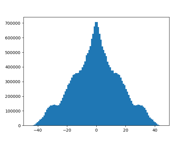
total_time = 500000  # Total simulation time (s)
γ = 1e-5 # friction

# Time array
t = np.arange(0, total_time, dt)
num_steps = len(t)

x = np.zeros(num_steps)
v = np.zeros(num_steps)
# Initial conditions
x[1] = x[0] = x_0
v[0] = v_0

α = np.exp(-γ*dt)
kbT = T # we don't actually have meaningful units for this exaple
scale = sqrt(kbT*(1-α**2)/m)
# Langevin Verlet's method loop
# v[i] and x[i] are offset by half dt
R = scale*np.random.normal(size=len(x))
for i in range(0,num_steps-1):
    v[i+1] = v[i]*α - (1-α)*k*x[i]/(γ*m) + R[i]
    x[i+1] = x[i] + v[i+1]*dt

velocities = (v[:-1]+v[1:])/2

plt.hist(x,bins=100)
plt.savefig('imgs/langevindist.png')

Overdamped Langevin (Brownian)
 $$\Large \color{red}{ m\frac{d^2x}{dt^2}}=\mathbf{F}-\gamma m \frac{dx}{dt} +\mathbf{R}$$
The Brownian equation of motion is derived from the Langevin equation of motion in the limit of large $\gamma$. In that case, the velocity of a particle is determined entirely by the instantaneous force acting on it, and kinetic energy ceases to have much meaning, since it disappears as soon as the applied force is removed. --openmm.org
$$\Large \frac{d{x}}{dt}=\frac{1}{\gamma m}\mathbf{F}+\frac{1}{\gamma m}\mathbf{R}$$
Fokker-Planck
Given a generic overdamped Langevin:
$$ \frac{dx}{dt} = -\frac{1}{m\gamma} \frac{dU}{dx} + \frac{1}{m\gamma} R(t)$$
the Fokker-Planck equation:
$$ \frac{\partial P}{\partial t} = \frac{1}{m\gamma}\frac{\partial}{\partial x} \left[ \frac{dU}{dx} P + k_BT \frac{\partial P}{\partial x} \right] $$
describes the evolution of a probability distribution $P$ under Langevin dynamics.
%%html
<div id="fpsolv" style="width: 500px"></div>
<script>
    var divid = '#fpsolv';
	jQuery(divid).asker({
	    id: divid,
	    question: "If I solve for dP/dt = 0, what probability distribution do you think we get?",
		answers: ["Uniform","Boltzmann","Normal","Unknown"],
        server: "https://bits.csb.pitt.edu/asker.js/example/asker.cgi",
		charter: chartmaker})

$(".jp-InputArea .o:contains(html)").closest('.jp-InputArea').hide();


</script>
Langevin dynamics has the Boltzmann distribution as its equilibrium distribution.
Limitations of Integration
- Molecular potentials are approximations.
- Lyapunov instability - minuscule differences in starting conditions can result in large differences in system evolution over time.
- This does not mean we can't effectively predict ensemble quantities.
$$\Large \boxed{ \text{Potential }U(x) \;\xrightarrow{-\nabla U}\; \text{forces} \;\xrightarrow{\text{integrator}}\; \text{trajectory} \;\xrightarrow{\text{sampling}}\; P(x) } $$
$$\Large \boxed{ P_{\rm eq}(x)\propto e^{-U(x)/k_BT} } $$
And now for something completely different the same