Practical MD I

Building a Simulation-Ready System

9/21/2026

print view

%%html
<script src="https://bits.csb.pitt.edu/preamble.js"></script>
<style>:root {--jp-cell-prompt-width: 32px}</style>

Homework 2

Why Molecular Dynamics?

To see how molecules move under some reasonable approximation of biological conditions.

• Does the drug bind?
• Is the protein stable?
• How does a mutation change the protein structure? Interactions?
• How are signals passed through the protein?
• What are the stable interactions?
• Do ions pass through the ion channel?
• What residues do what to achieve the protein's function?

Ion Channels

Second largest class of drug targets.

NMDA receptor (5UN1)	GABAA receptor (6X3T)
MK-801 (memantine mimic)	propofol
Alzheimer's	anaesthetic

https://www.guidetopharmacology.org/

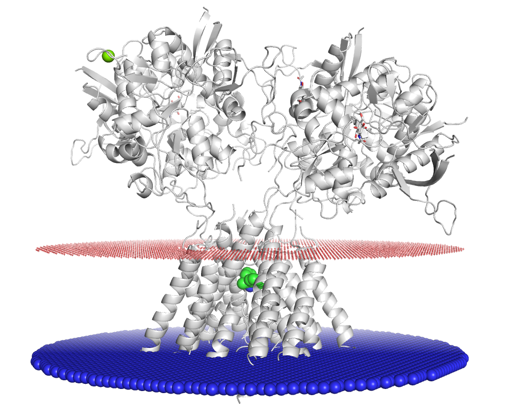
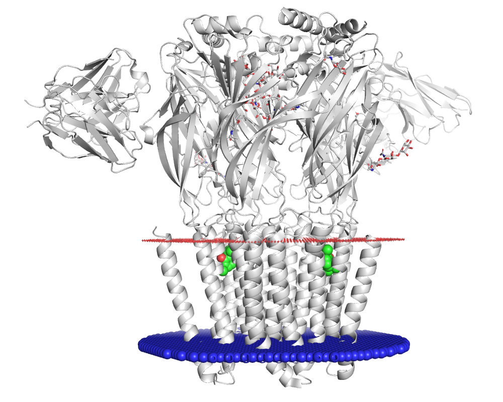
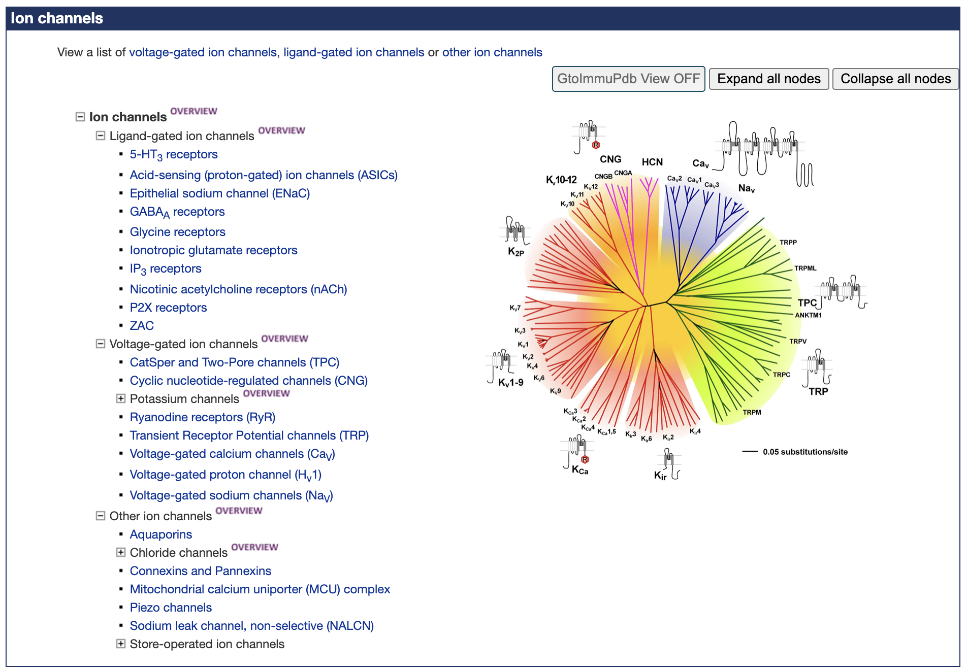
%%html
<div id="structmd1" style="width: 500px"></div>
<script>
$('head').append('<link rel="stylesheet" href="https://bits.csb.pitt.edu/asker.js/themes/asker.default.css" />');

    var divid = '#structmd1';
	jQuery(divid).asker({
	    id: divid,
	    question: "Assuming sufficient simulation time, which of the following processes can <b>not</b> be observed in a molecular dynamics simulation?",
        answers: ["Unbinding","Folding","Transcription","Residue Conformations"],
		extra: ["The disassociation of two proteins",'The folding of a protein','The construction of RNA by RNA polymerase',
                 'The conformational sampling of residue side chains or short loop regions '],
        server: "https://bits.csb.pitt.edu/asker.js/example/asker.cgi",
		charter: chartmaker})
    
$(".jp-InputArea .o:contains(html)").closest('.jp-InputArea').hide();


</script>

What MD actually propagates

The dynamical state contains positions and velocities. At each step an integrator updates both according to the chosen equations of motion.

$$U(\mathbf{x}) \rightarrow \mathbf{F}(\mathbf{x})=-\nabla U(\mathbf{x}) \rightarrow (\mathbf{x}_{t+\Delta t},\mathbf{v}_{t+\Delta t})$$

Two separate limitations matter:

1. The model: standard fixed-topology classical MD cannot change chemical connectivity.
2. The sampling: a process can be allowed by the model but still occur on a timescale far longer than the trajectory.

So “can MD describe it?” and “will I observe it?” are different questions.

Lindorff-Larsen K, Piana S, Dror RO, Shaw DE. How fast-folding proteins fold. Science. 2011 Oct 28;334(6055):517-20.

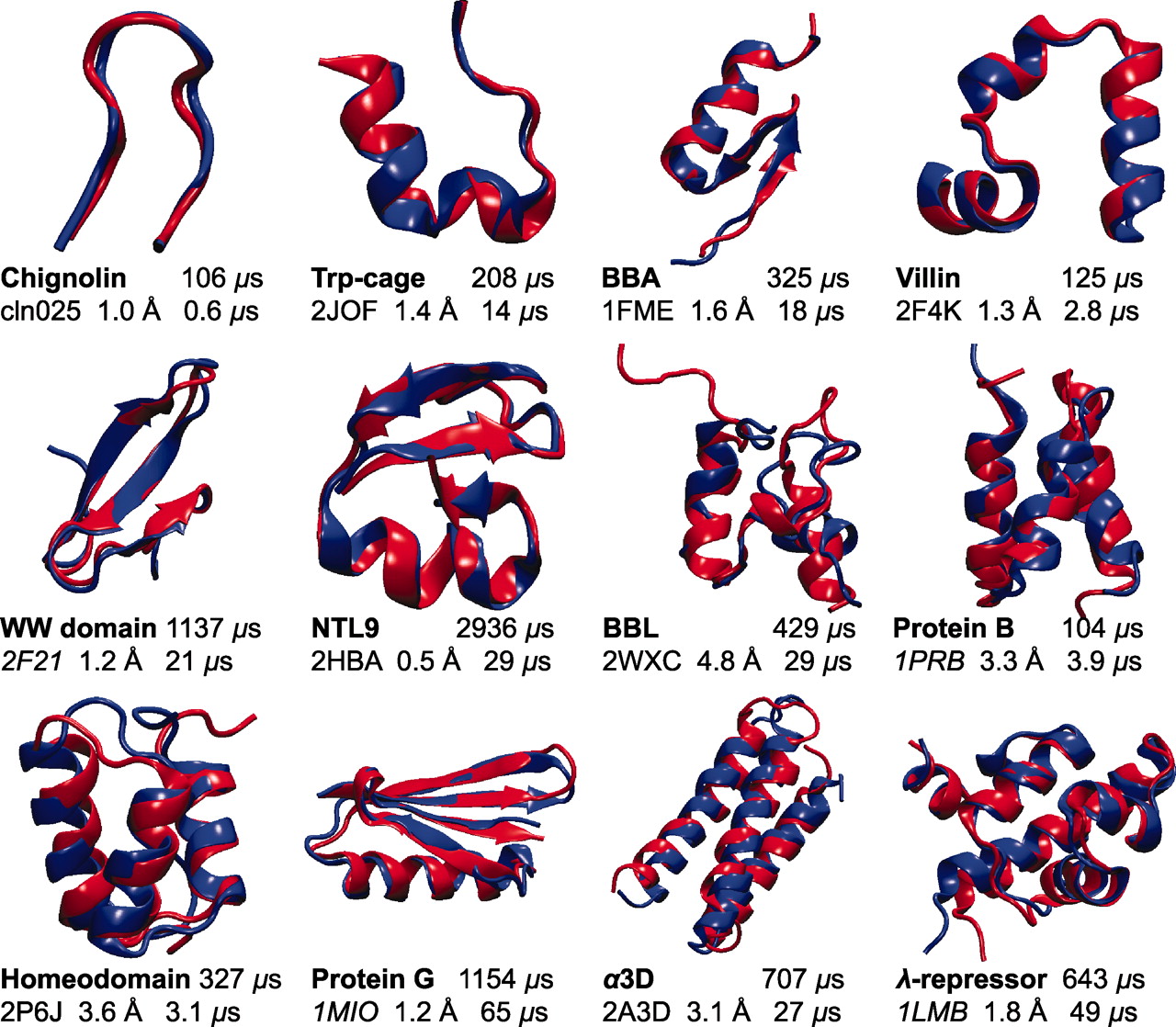
Basic Approach

• Initialize system
• $t \leftarrow 0$
• For $N$ steps:
  • calculate forces for current positions
  • integrate equations of motion to update positions/velocities
  • output quantities of interest
  • $t \leftarrow t + \Delta t$

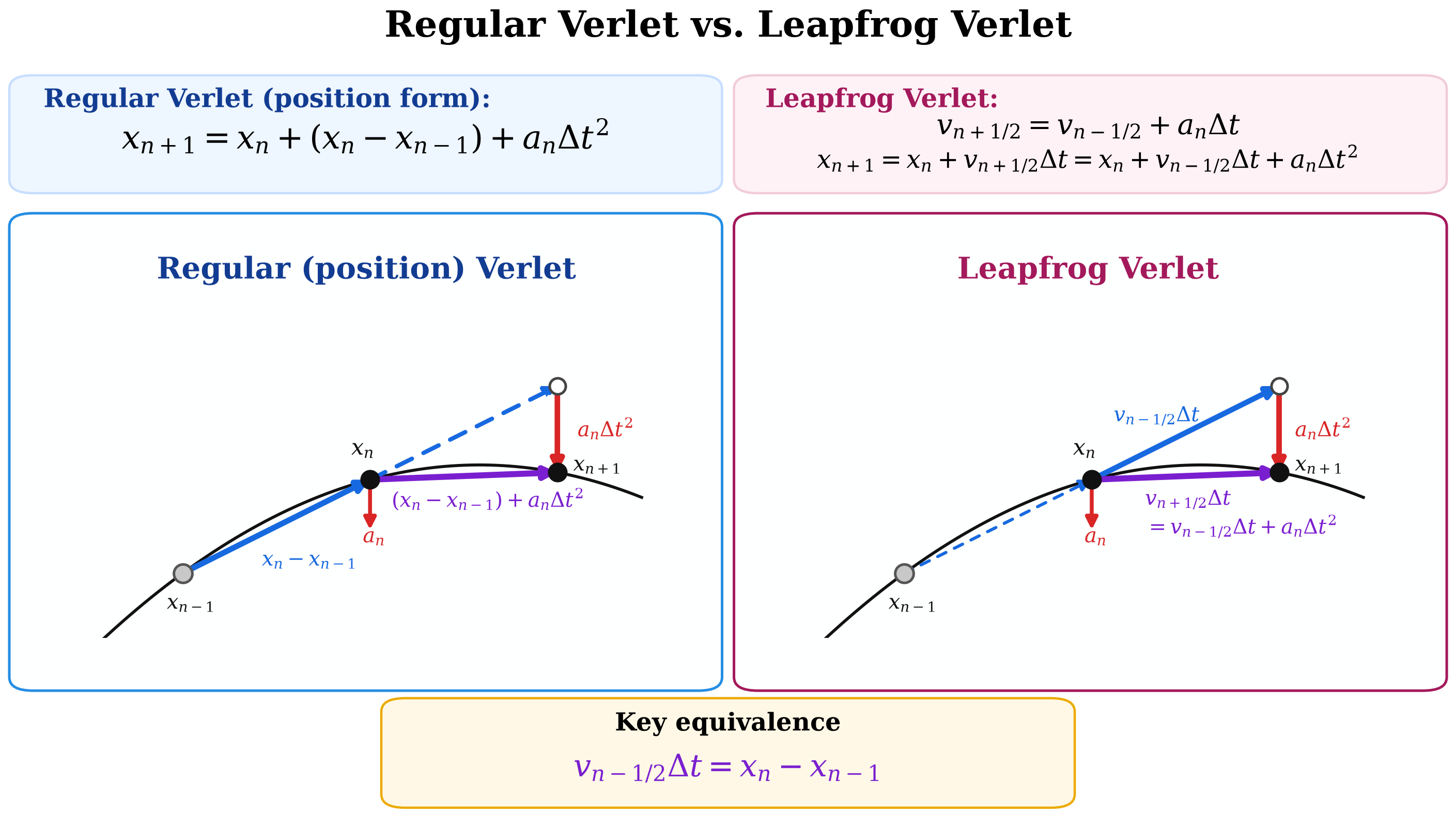
MD Packages

Amber http://ambermd.org

• Fastest GPU implementation (in my experience)

Gromacs http://www.gromacs.org

• Open-source (LGPL)

NAMD http://www.ks.uiuc.edu/Research/namd/

• Highly optimized for cluster computing
• Integrated with VMD

LAMMPS http://lammps.sandia.gov

• Open-source (GPL)

OpenMM https://openmm.org/

• Open-source
• Python interface
• Most modern

Initializing the system

What molecule(s) to simulate?

Solvent? Salts?

What size box and under what conditions?

Before adding water: define the molecular model

Ask first:

• Which biological assembly, chains, ligands, cofactors, waters, and ions belong?
• Are residues/atoms missing? Are alternate conformations present?
• What are the termini, disulfides, protonation states, and histidine tautomers?
• Are there mutations or engineered residues?
• Is a ligand/cofactor already covered by the chosen force field?

import py3Dmol
import openmm
from openmm.app import *
from openmm.unit import *

Fixing problems

If the input contains unresolved chemistry or missing atoms, system builders may fail—or worse, may produce a system that runs but is not the system you intended.

protein = PDBxFile('data/1qg8.cif')
mmodeller = Modeller(protein.topology, protein.positions)
forcefield = ForceField('amber14-all.xml', 'amber14/tip3p.xml')
mmodeller.addSolvent(forcefield)

---------------------------------------------------------------------------
ValueError                                Traceback (most recent call last)
Cell In[5], line 4
      1 protein = PDBxFile('data/1qg8.cif')
      2 mmodeller = Modeller(protein.topology, protein.positions)
      3 forcefield = ForceField('amber14-all.xml', 'amber14/tip3p.xml')
----> 4 mmodeller.addSolvent(forcefield)

File ~/Library/Python/3.14/lib/python/site-packages/openmm/app/modeller.py:524, in Modeller.addSolvent(self, forcefield, model, boxSize, boxVectors, padding, numAdded, boxShape, positiveIon, negativeIon, ionicStrength, neutralize, residueTemplates)
    520         raise ValueError('Neither the box size, box vectors, nor padding was specified, and the Topology does not define unit cell dimensions')
    522 # Have the ForceField build a System for the solute from which we can determine van der Waals radii.
--> 524 system = forcefield.createSystem(self.topology, residueTemplates=residueTemplates)
    525 nonbonded = None
    526 for i in range(system.getNumForces()):

File ~/Library/Python/3.14/lib/python/site-packages/openmm/app/forcefield.py:1305, in ForceField.createSystem(self, topology, nonbondedMethod, nonbondedCutoff, constraints, rigidWater, removeCMMotion, hydrogenMass, residueTemplates, ignoreExternalBonds, switchDistance, flexibleConstraints, drudeMass, **args)
   1301 rigidResidue = [False]*topology.getNumResidues()
   1303 # Find the template matching each residue and assign atom types.
-> 1305 templateForResidue = self._matchAllResiduesToTemplates(data, topology, residueTemplates, ignoreExternalBonds)
   1306 for res, template in templateForResidue.items():
   1307     if res.name == 'HOH':
   1308         # Determine whether this should be a rigid water.

File ~/Library/Python/3.14/lib/python/site-packages/openmm/app/forcefield.py:1578, in ForceField._matchAllResiduesToTemplates(self, data, topology, residueTemplates, ignoreExternalBonds, ignoreExtraParticles, recordParameters)
   1576                 break
   1577 if matches is None:
-> 1578     raise ValueError('No template found for residue %d (%s).  %s  For more information, see https://github.com/openmm/openmm/wiki/Frequently-Asked-Questions#template' % (res.index, res.name, _findMatchErrors(self, res)))
   1579 else:
   1580     if res in unmatchedResidues:

ValueError: No template found for residue 0 (PRO).  The set of heavy atoms matches PRO, but the residue is missing 7 H atoms.  You may be able to add them with Modeller.addHydrogens().  For more information, see https://github.com/openmm/openmm/wiki/Frequently-Asked-Questions#template

PDBFixer

Uses simple heuristic algorithms to fix common problems. Always inspect the resulting structure.

from pdbfixer.pdbfixer import PDBFixer
fixer = PDBFixer('data/1qg8.cif')
fixer.removeHeterogens(False) # remove water and ions
fixer.findMissingResidues()
fixer.findMissingAtoms()
fixer.addMissingAtoms()
fixer.addMissingHydrogens(7.0)

fixer.missingResidues

{(0, 132): ['GLU', 'ASN', 'ARG'],
 (0, 213): ['ASP',
  'GLN',
  'SER',
  'ILE',
  'HIS',
  'PHE',
  'GLN',
  'LEU',
  'PHE',
  'GLU',
  'LEU',
  'GLU',
  'LYS',
  'ASN']}

with open('fixed.pdb', 'w') as outfile:
    PDBFile.writeFile(fixer.topology, fixer.positions, outfile)

v = py3Dmol.view(data=open('data/1qg8.cif').read()); v.addModel(open('fixed.pdb').read())
v.setStyle('cartoon');v.setStyle({'model':1,'resi':'216-231'},{'cartoon':{'colorscheme':'greenCarbon'},'stick':{'colorscheme':'greenCarbon'}})
v.zoomTo({'resi':'216-231'}).show()

3Dmol.js failed to load for some reason. Please check your browser console for error messages.

Missing residues: automation is not evidence

PDBFixer can generate coordinates for missing residues. That is useful, but the generated conformation is a model, not experimental information.

For a long unresolved loop ask:

• Was the region absent because it is flexible/disordered?
• Is rebuilding it necessary for the scientific question?
• Does it interact with the region we care about?
• Should alternative models or restraints be considered?

Always inspect the result.

Molecular System File Formats

MD codes separate the representation of a molecular system into a topology (what the atoms are and how they are connected) and coordinates (the positions of the atoms). A PDB can represent both, but poorly.

Topology Formats

• .prmtop - Amber
• .psf - NAMD
• .top - Gromacs

Coordinate Formats

• .pdb - Gromacs, NAMD
• .inpcrd - Amber
• .rst - Amber Restart

Five objects to keep straight

Object	What it represents	Examples
Topology	what atoms exist and how they are connected	PDB/mmCIF topology, PSF
Parameterized system	the energy function: masses, charges, force-field parameters, constraints	Amber prmtop, OpenMM System
Coordinates	one configuration: where the atoms are	PDB/mmCIF, Amber inpcrd
Trajectory	coordinates sampled over time	DCD, XTC, NetCDF trajectory
Checkpoint / restart	enough simulation state to continue a run	OpenMM checkpoint, Amber restart

A molecular configuration is not fully defined by coordinates alone:

$$ \text{topology} + \text{parameters} + \text{coordinates} \;\longrightarrow\; U(\mathbf{x}) $$

For analysis, we usually combine a topology + trajectory.

Solvent

Most of our time is spent simulating water, so simplified representations are desirable.

Forcefields are typically calibrated for a specific water model - use that one.

TIP3P (Transferable Interaction Potential 3-point model)

• 3 point charges (-0.834, +0.417)
• bond lengths kept fixed (0.9572$\unicode{x212B}$)
• angle kept fixed ($104.52^\circ$)
• Lennard-Jones (van der Waals) calculated only for O

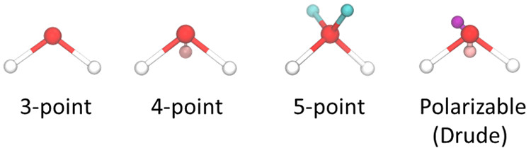
J. Chem. Inf. Model. 2021, 61, 9, 4521-4536

SPC / SPC-E

• SPC = Simple Point Charge
• Rigid, 3-site water model, like TIP3P
  • charges are located on the O and H atoms
  • Lennard-Jones interaction is centered on O
• Similar computational cost to TIP3P
• SPC/E modifies the charges and includes an average polarization-energy correction
• SPC/E generally reproduces bulk liquid properties better than the original SPC model

OPC

• OPC = Optimal Point Charge
• Rigid, 4-site water model
  • positive charges on the H atoms
  • negative charge on a massless virtual site near the oxygen
  • Lennard-Jones interaction is centered on O
• Charge locations were optimized to reproduce the electrostatics of water
• Designed to reproduce a broad range of bulk-water properties more accurately than older 3-site models

Salts

Typically need to neutralize system.

Biologically, don't expect molecules to be in pure water.

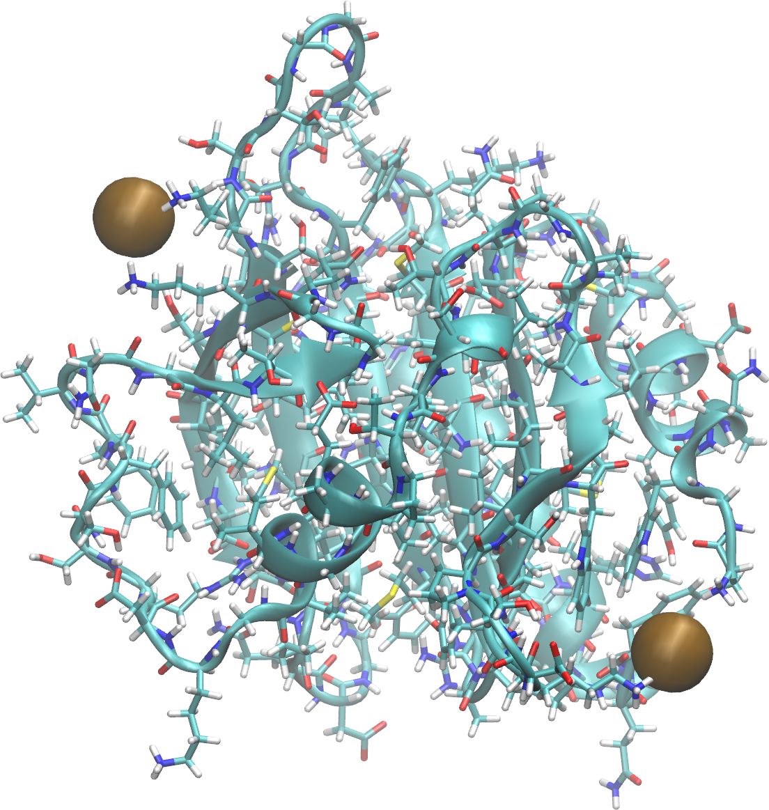
%%html
<div id="ionq" style="width: 500px"></div>
<script>
$('head').append('<link rel="stylesheet" href="https://bits.csb.pitt.edu/asker.js/themes/asker.default.css" />');

    var divid = '#ionq';
	jQuery(divid).asker({
	    id: divid,
	    question: "What ion are the brown spheres on the previous slide?",
		answers: ["Cl-","Na+"],
        server: "https://bits.csb.pitt.edu/asker.js/example/asker.cgi",
		charter: chartmaker})
    
$(".jp-InputArea .o:contains(html)").closest('.jp-InputArea').hide();


</script>

Are they sufficient to neutralize the system?

The Box

Typically want a buffer of 8-12$\unicode{x212B}$ around protein.

But also want to avoid simulating water molecules far from protein, so use more compact "box" shapes.

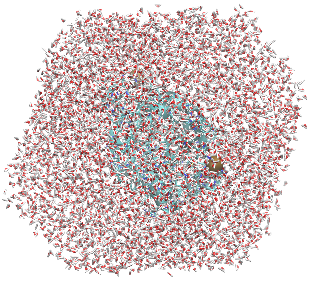
Truncated octahedron.

Periodic Boxes

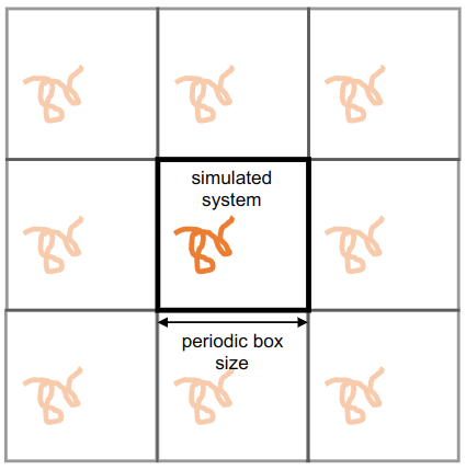
We simulate in a periodic box. This better represents the behavior in a larger "bulk phase"

• Not a nanodroplet in space
• There are no physical walls; an atom crossing one face re-enters through the opposite face
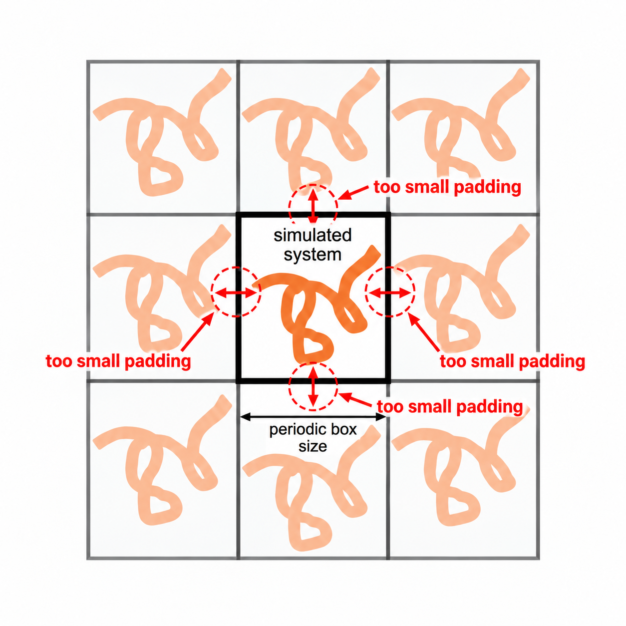
• Important to have sufficient buffer (padding) that molecule doesn't interact with itself
• Periodicity is implemented in the force calculation

Setting up a system

import py3Dmol
import openmm
from openmm.app import *
from openmm.unit import *

modeller = Modeller(Topology(),[])
forcefield = ForceField('amber14-all.xml', 'amber14/tip3p.xml')
modeller.addSolvent(forcefield,boxSize=(5,5,5),ionicStrength=.01*molar)

import io

def show(topology, positions):
    out = io.StringIO()
    PDBFile.writeFile(topology,positions, out)
    v = py3Dmol.view()
    v.addModel(out.getvalue(),'pdb',{'keepH':True})
    v.setStyle('sphere')
    v.setStyle({'resn':'HOH'},'stick')
    v.zoomTo()
    return v.show()

show(modeller.topology, modeller.positions)

3Dmol.js failed to load for some reason. Please check your browser console for error messages.

Solvent Box Options

addSolvent(forcefield, model='tip3p', boxSize=None, boxVectors=None, padding=None, numAdded=None, boxShape='cube', positiveIon='Na+', negativeIon='Cl-', ionicStrength=Quantity(value=0, unit=molar), neutralize=True)

• Can set kind of ion
  • Cs+, K+, Li+, Na+, Rb+
  • Cl-, Br-, F-, and I-
• Default is to neutralize - add only as many ions as needed (so none, all positive, all negative)
• If ionic strength is set, will add pairs of ions to achieve target
• Can specify the size and shape of the box
  • dimensions are assumed nanometers
  • or set numAdded and it will size a cubic box with that many molecules
  • specify padding - will create box with at least this much space around the solute
    • recommend 12$\unicode{x212B}$

Padding Periodic Boxes

The padding should be sufficient to prevent the solute from making direct short-range contacts with its nearest periodic image.

modeller = Modeller(Topology(),[]); forcefield = ForceField('amber14-all.xml', 'amber14/tip3p.xml')
modeller.addSolvent(
    forcefield,
    boxShape='octahedron',
    padding=1.2*nanometer,   # 12 Å
    ionicStrength=.01*molar)
show(modeller.topology, modeller.positions)

3Dmol.js failed to load for some reason. Please check your browser console for error messages.

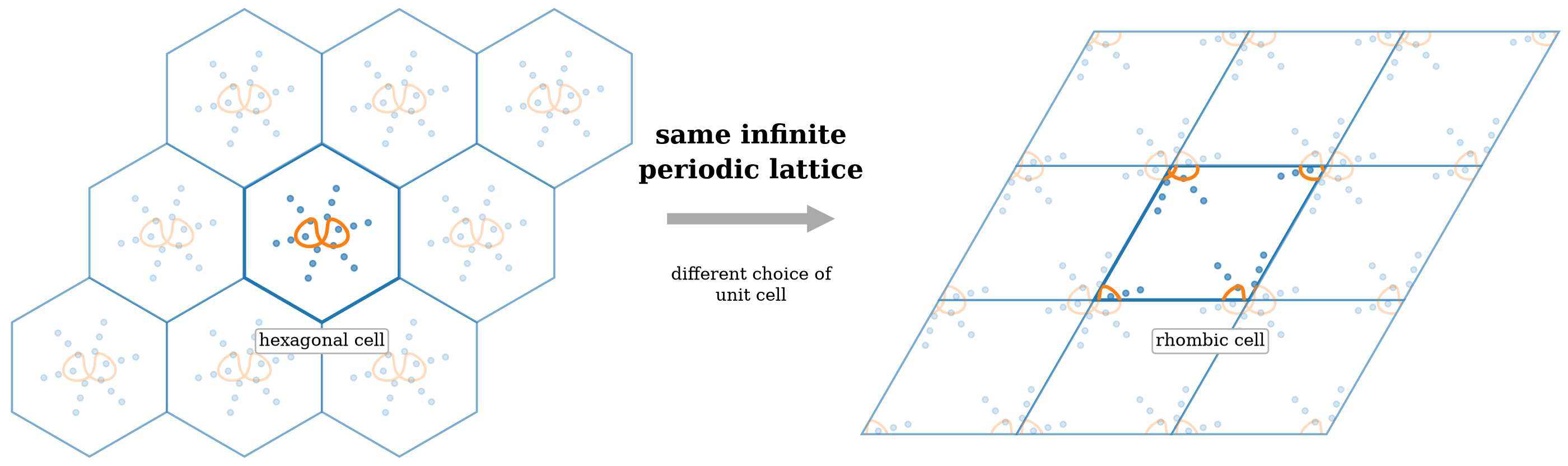
More than one way to tile the same periodic system...

Solvent Adding Algorithm

1. Water molecules are added to fill the box using a predefined template.
2. Water molecules are removed if their distance to any solute atom is less than the sum of their van der Waals radii (overlapping).
3. If the solute is charged and neutralize=True, enough positive or negative ions are added to neutralize it. Each ion is added by randomly selecting a water molecule and replacing it with the ion.
4. Ion pairs are added to give the requested total ionic strength.

Does this algorithm result in an ideally solvated system?

The water template

v = py3Dmol.view(); v.addModel(open(openmm.__path__[0]+'/app/data/tip3p.pdb').read(),'pdb',{'keepH':True}); v.setStyle('stick'); v.zoomTo(); v.show()

3Dmol.js failed to load for some reason. Please check your browser console for error messages.

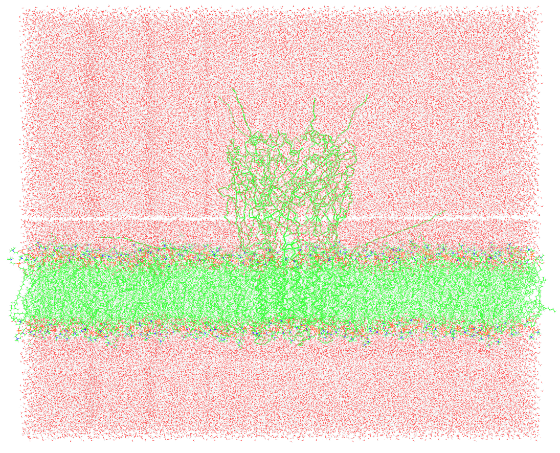
Adding more than just water

from pdbfixer.pdbfixer import PDBFixer
fixer = PDBFixer('data/5tin.pdb')
fixer.findMissingResidues()
fixer.findMissingAtoms()
fixer.addMissingAtoms()
fixer.addMissingHydrogens(7.0)

mmodeller = Modeller(fixer.topology, fixer.positions)
mmodeller.addMembrane(forcefield,lipidType='POPC',minimumPadding=1*nanometer)

PDBxFile.writeFile(mmodeller.topology, mmodeller.positions, 'membrane.cif')

Force fields

A force field specifies the potential-energy function $U(\mathbf{x})$ and its parameters. Forces follow from

$$\mathbf{F}(\mathbf{x})=-\nabla U(\mathbf{x}).$$

Examples of force-field families include:

• CHARMM
• GROMOS
• OPLS
• AMBER

Different families—and sometimes variants within a family—can differ in both functional form and parameterization: torsions, 1–4 treatment, combining rules, CMAP/Urey-Bradley terms, charge models, etc.

Amber

$$U(r^N)=\sum_\text{bonds} k_b (l-l_0)^2 + \sum_\text{angles} k_a (\theta - \theta_0)^2 + \sum_\text{torsions} \frac{1}{2} U_n [1+\cos(n \omega- \gamma)] $$ $$+\sum_{j=1} ^{N-1} \sum_{i=j+1} ^N \biggl\{\epsilon_{i,j}\biggl[\left(\frac{r_{0ij}}{r_{ij}} \right)^{12} - 2\left(\frac{r_{0ij}}{r_{ij}} \right)^{6} \biggr]+ \frac{q_iq_j}{4\pi \epsilon_0 r_{ij}}\biggr\} $$

Note that non-bonded interactions are only calculated for atoms separated by more than 3 bonds (or are scaled down for "1-4" interactions).

Bond Stretch

Folmsbee DL, Koes DR, Hutchison GR. Evaluation of thermochemical machine learning for potential energy curves and geometry optimization. The Journal of Physical Chemistry A. 2021 Feb 25;125(9):1987-93.

 forcefield.getGenerators()

[<openmm.app.forcefield.HarmonicBondGenerator at 0x111f30690>,
 <openmm.app.forcefield.HarmonicAngleGenerator at 0x119300a50>,
 <openmm.app.forcefield.NonbondedGenerator at 0x119300b90>,
 <openmm.app.forcefield.PeriodicTorsionGenerator at 0x119301310>]

%%html
<div id="nonbondq" style="width: 500px"></div>
<script>
$('head').append('<link rel="stylesheet" href="https://bits.csb.pitt.edu/asker.js/themes/asker.default.css" />');

    var divid = '#nonbondq';
	jQuery(divid).asker({
	    id: divid,
	    question: "Consider two atoms in a protein that are far apart in the covalent bonding graph but close together in 3D space. Which force-field terms can directly describe their interaction?",
        answers: ["Bonds/angles","Torsions ","Nonbonded","None"],
		extra: ["Bond and angle terms only",'Torsional terms only','Lennard-Jones and electrostatic terms',
                 'No interaction, because they are not covalently bonded'],
        server: "https://bits.csb.pitt.edu/asker.js/example/asker.cgi",
		charter: chartmaker})
    
$(".jp-InputArea .o:contains(html)").closest('.jp-InputArea').hide();


</script>

Assignment 2 revisited: decompose the torsion scan

Instead of recording only the total energy at each rigid dihedral angle, assign each OpenMM force term to a force group and record them separately:

from openmm.openmm import Platform, VerletIntegrator, LangevinIntegrator, AndersenThermostat
import matplotlib.pyplot as plt 

# read file
pdb = PDBFile('data/gly.pdb')

# setup openmm system using amber 14 forcefield which defines the potential energy function
ff = ForceField('amber14-all.xml')
system = ff.createSystem(pdb.topology,ignoreExternalBonds=True)

# Assign force groups
energies = {}
group = {}
for i, force in enumerate(system.getForces()):
    force.setForceGroup(i)
    group[force.__class__.__name__] = i
    energies[force.__class__.__name__] = []
    
# we aren't actually simulating, but need a simulation object to calculate energies
integrator = VerletIntegrator(1*femtosecond)
simulation = Simulation(pdb.topology, system, integrator)

# store atom positions
# note that more code is necessary for this code to be a general solution
# as opposed to only working with our carefully prepared inputs
origpos = np.array(pdb.getPositions()._value)
newpos = origpos.copy()

capos = origpos[1]
cpos = origpos[2]

# a boolean mask of the atoms that should be rotated around the dihedral
mask = moving_atoms(pdb, 1, 2)

angles = []
total = []
for d in range(0,360,1):
    # rotate atoms
    R = make_rotation_matrix(capos,cpos,np.deg2rad(d))    
    newpos[mask] = np.matmul(R,origpos[mask].T).T
     
    # setPositions to newpos in simulation (TODO)
    simulation.context.setPositions(newpos)
    
    for i, force in enumerate(system.getForces()):
        name = force.__class__.__name__
        state = simulation.context.getState(getEnergy=True, groups={group[name]})
        energies[name].append(state.getPotentialEnergy())
    
    # get simulation.context state, fetching energy
    state = simulation.context.getState(getEnergy=True)
    total.append(state.getPotentialEnergy())
    # record the dihedral
    d = dihedral(*newpos[:4])
    if d < 0: d += 2*np.pi
    angles.append(np.rad2deg(d))
    

plt.figure(figsize=(8,6))
for k in energies.keys():
    plt.plot(angles,[e.value_in_unit(kilojoule_per_mole) for e in energies[k]],label=k)
plt.legend(loc='best',ncol=3); plt.ylabel("Energy (kJ/mol)"); plt.xlabel("Dihedral (Degrees)"); plt.ylim(0,12);

CHARMM

$$U(r^N)=\sum_{bonds}k_b(b-b_0)^2+\sum_{angles}k_{\theta}(\theta-\theta_0)^2+\sum_{dihedrals}k_\phi[1+\cos(n\phi-\delta)]$$ $$+\sum_{impropers}k_\omega(\omega-\omega_0)^2+\sum_{Urey-Bradley}k_u(u-u_0)^2 $$ $$+\sum_{nonbonded}\left(\epsilon_{ij}\left[\left(\frac{R_{min_{ij}}}{r_{ij}}\right)^{12}-2\left(\frac{R_{min_{ij}}}{r_{ij}}\right)^6\right]+\frac{q_i q_j}{\epsilon_r r_{ij}}\right) $$

The Urey-Bradley term is an explicit bonded harmonic potential on the 1–3 distance associated with an angle; it is not an ordinary nonbonded interaction.

Modern CHARMM protein force fields also include correction terms such as CMAP (correction map).

charm = ForceField('charmm36.xml')
charm.getGenerators()

[<openmm.app.forcefield.HarmonicBondGenerator at 0x1506956d0>,
 <openmm.app.forcefield.HarmonicAngleGenerator at 0x150695310>,
 <openmm.app.forcefield.AmoebaUreyBradleyGenerator at 0x153893a10>,
 <openmm.app.forcefield.PeriodicTorsionGenerator at 0x150694cd0>,
 <openmm.app.forcefield.CustomTorsionGenerator at 0x1538930e0>,
 <openmm.app.forcefield.CMAPTorsionGenerator at 0x153893cb0>,
 <openmm.app.forcefield.NonbondedGenerator at 0x152294190>,
 <openmm.app.forcefield.LennardJonesGenerator at 0x153893620>]

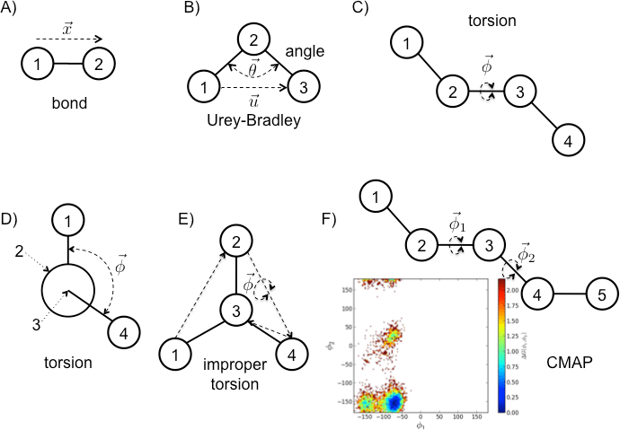
Swails, Jason. (2013). Free Energy Simulations of Complex Biological Systems at Constant pH. 10.13140/2.1.4501.1844.

Let's look at a force field definition

Amber14sb

What force field to use?

Most common answer to "why did you choose that force field?"

It's what my advisor/mentor uses

I recommend AMBER ff15ipq + SPC/E water model.

• Good match to experimental (NMR) observables
• Developed at Pitt

What about drugs?

A protein force field does not automatically parameterize a novel ligand.

A realistic drug-discovery system may require:

• protein/nucleic-acid force field
• compatible water and ion parameters
• small-molecule parameters and partial charges (for example GAFF- or OpenFF-style models)
• special treatment for metals, covalent ligands, unusual residues, or cofactors

If the chemistry is not parameterized, the simulation does not yet have a defined $U(\mathbf{x})$.

Efficiency Considerations

The most expensive part of MD is calculating the non-bonded forces.

$$\sum_{j=1} ^{N-1} \sum_{i=j+1} ^N \biggl\{\epsilon_{i,j}\biggl[\left(\frac{r_{0ij}}{r_{ij}} \right)^{12} - 2\left(\frac{r_{0ij}}{r_{ij}} \right)^{6} \biggr]+ \frac{q_iq_j}{4\pi \epsilon_0 r_{ij}}\biggr\} $$

Why?

Also, are these forces?

Cutoffs increase efficiency

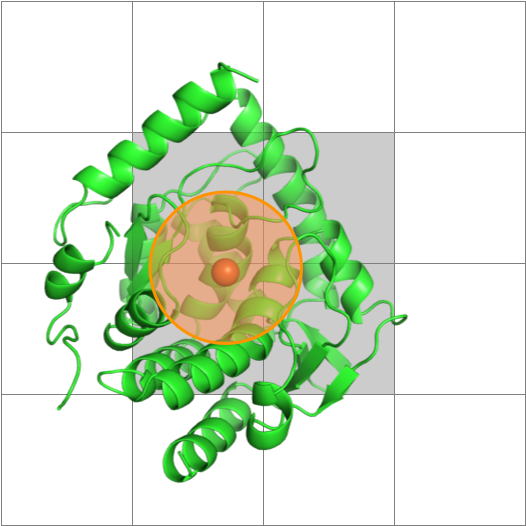
Maintain a list of neighbors within the cutoff and calculate short-range forces only for those pairs.

• A naive neighbor-list rebuild would be $O(N^2)$.
• Voxelize space (spatial decomposition) and only calculate atoms in adjacent voxels.
• In practice do both: use voxels (cell lists) to update neighbor lists, then evaluate only listed pairs.

#make a larger water box
from openmm.openmm import Platform, VerletIntegrator, LangevinIntegrator, AndersenThermostat
platform = Platform.getPlatformByName('Reference')
modeller = Modeller(Topology(),[])
forcefield = ForceField('amber14-all.xml', 'amber14/tip3p.xml')
modeller.addSolvent(forcefield,boxSize=(6,6,6),ionicStrength=.01*molar)

system = forcefield.createSystem(modeller.topology,  nonbondedMethod=NoCutoff)
simulation = Simulation(modeller.topology, system, VerletIntegrator(1*femtosecond),platform=platform)
simulation.context.setPositions(modeller.positions)
modeller.topology

<Topology; 2 chains, 7128 residues, 21380 atoms, 14252 bonds>

%%time
simulation.step(10)

CPU times: user 42.2 s, sys: 90.1 ms, total: 42.3 s
Wall time: 42.4 s

system = forcefield.createSystem(modeller.topology,  nonbondedMethod=CutoffNonPeriodic,
                                 nonbondedCutoff=1*nanometer)
simulation = Simulation(modeller.topology, system, VerletIntegrator(1*femtosecond),platform=platform)
simulation.context.setPositions(modeller.positions)

%%time
simulation.step(10)

CPU times: user 2.15 s, sys: 3.9 ms, total: 2.16 s
Wall time: 2.16 s

Long-range electrostatics in a periodic system

Simply truncating Coulomb interactions is a poor model of long-range electrostatics.

Ewald-family methods split the problem into

$$E = E_{\text{short range}} + E_{\text{long range}} + E_{\text{self correction}}$$

Particle Mesh Ewald (PME) evaluates the long-range part efficiently with a mesh + FFT, giving roughly $O(N\log N)$ scaling.

For routine biomolecular simulations, the practical takeaway is: use a periodic electrostatics method such as PME rather than treating Coulomb interactions as purely local.

Particle Mesh Ewald

CutoffNonPeriodic sets forces to zero after the cutoff.

Ewald, PME, or LJPME assume a periodic box. To compute the interactions of the full periodic system, interactions are separated into short-range "direct space" calculations (less than cutoff) and long-range reciprocal space (Fourier transform).

$$E=E_{\mathit{dir}}+{E}_{\mathit{rec}}+{E}_{\mathit{self}}$$ $$E_{\mathit{dir}}=\frac{1}{2}\sum _{i,j}\sum_\mathbf{n}{q}_{i}{q}_{j}\frac{\text{erfc}\left({\mathit{\alpha r}}_{ij,\mathbf{n}}\right)}{r_{ij,\mathbf{n}}}$$ $$E_{\mathit{rec}}=\frac{1}{2{\pi}V}\sum _{i,j}q_i q_j\sum _{\mathbf{k}{\neq}0}\frac{\text{exp}(-(\pi \mathbf{k}/\alpha)^2+2\pi i \mathbf{k} \cdot (\mathbf{r}_{i}-\mathbf{r}_{j}))}{\mathbf{k}^2}$$ $$E_{\mathit{self}}=-\frac{\alpha}{\sqrt{\pi}}\sum _{i}{q}_{i}^{2}$$

Derivation

Particle Mesh Ewald uses a Fast Fourier Transform to achieve $O(N \log N)$ scaling while computing the (approximate) electrostatic energy for the entire periodic system.

Constraints

The fastest motions in an all-atom biomolecular model are typically bonds involving hydrogen.

If we constrain those bond lengths rather than integrating their vibrations, we can take a larger timestep.

• unconstrained fast bonds → roughly 1 fs scale
• X-H bond constraints → 2 fs is a conservative default
• larger timesteps can be possible with suitable integrators/constraint strategies and should be validated

Constraints change which degrees of freedom are explicitly simulated; they are not merely a software speed setting.

system = forcefield.createSystem(modeller.topology,  
                                 nonbondedMethod=PME,
                                 constraints=HBonds)

Energy Minimization

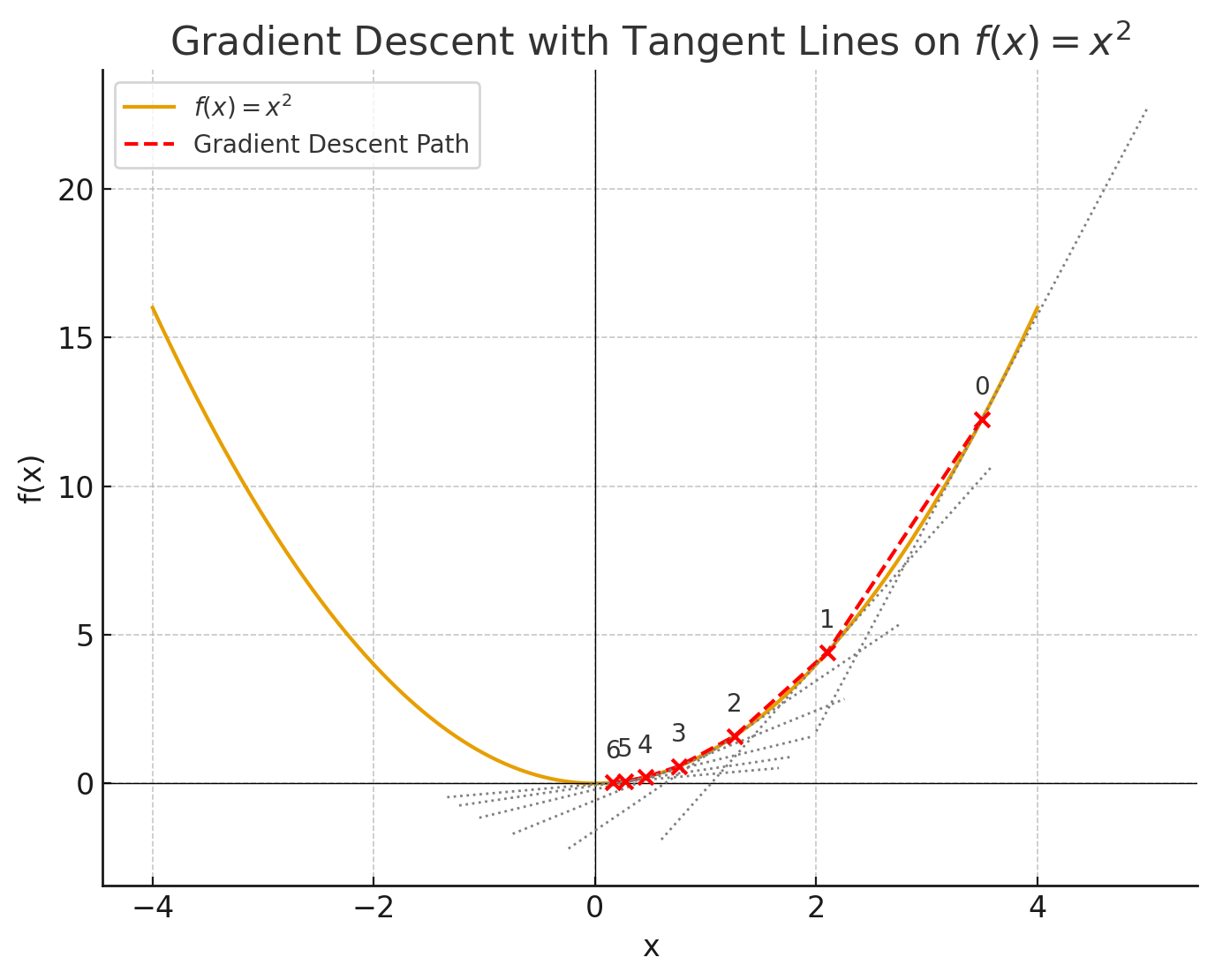Before runing a simulation, energy minimize the system to resolve any local issues (e.g. clashes) that might cause the system to "blow up".

• May need also run energy minimization before solvating protein. Why?

Recall our fixed up protein...

from pdbfixer.pdbfixer import PDBFixer
fixer = PDBFixer('data/1qg8.cif')
fixer.removeHeterogens(False) # remove water and ions
fixer.findMissingResidues(); fixer.findMissingAtoms()
fixer.addMissingAtoms(); fixer.addMissingHydrogens(7.0)
with open('fixed.pdb', 'w') as outfile:
    PDBFile.writeFile(fixer.topology, fixer.positions, outfile)
    

v = py3Dmol.view(data=open('data/1qg8.cif').read()); v.addModel(open('fixed.pdb').read())
v.setStyle('cartoon');v.setStyle({'model':1,'resi':'216-231'},{'cartoon':{'colorscheme':'greenCarbon'},'stick':{'colorscheme':'greenCarbon'}})
v.zoomTo({'resi':'216-231'}).show()

3Dmol.js failed to load for some reason. Please check your browser console for error messages.

ff = ForceField('amber14-all.xml')
system = ff.createSystem(fixer.topology,  nonbondedMethod=PME,constraints=HBonds)
simulation = Simulation(fixer.topology, system, VerletIntegrator(2*femtosecond))
simulation.context.setPositions(fixer.positions)
state = simulation.context.getState(getEnergy=True)
print("Original Energy:",state.getPotentialEnergy())
simulation.minimizeEnergy()
state = simulation.context.getState(getEnergy=True,getPositions=True)
print("Minimized Energy:",state.getPotentialEnergy())

Original Energy: 85165016857.326 kJ/mol
Minimized Energy: -32449.176259411484 kJ/mol

v = py3Dmol.view(data=open('fixed.pdb').read()); v.addModel(open('minimized.pdb').read()); v.setStyle({'model':0,'resi':'216-231'},{'stick':{'colorscheme':'greenCarbon','radius':.15}}); v.setStyle({'model':1,'resi':'216-231'},{'stick':{'colorscheme':'yellowCarbon'}}); v.zoomTo({'resi':'216-231'}).show()

3Dmol.js failed to load for some reason. Please check your browser console for error messages.

Here, the energy minimization is part of our initial model construction, rather than a pre-simulation refinement.

System setup

modeller = Modeller(fixer.topology, state.getPositions())
forcefield = ForceField('amber14/protein.ff15ipq.xml', 'amber14/spce.xml')
modeller.addSolvent(forcefield, padding=1.0*nanometer,model='spce',boxShape='octahedron')

system = forcefield.createSystem(modeller.topology, nonbondedMethod=PME, 
                    nonbondedCutoff=1*nanometer,  constraints=HBonds)
integrator = VerletIntegrator(2*femtosecond)
simulation = Simulation(modeller.topology, system, integrator)
simulation.context.setPositions(modeller.positions)

state = simulation.context.getState(getEnergy=True,getPositions=True)
print("Unminimized Energy:",state.getPotentialEnergy())
# Energy minimize
simulation.minimizeEnergy()

Unminimized Energy: -205127.25301367324 kJ/mol

state = simulation.context.getState(getEnergy=True,getPositions=True)
print("Minimized Energy:",state.getPotentialEnergy())

Minimized Energy: -452258.69051367324 kJ/mol

show(modeller.topology,simulation.context.getState(getPositions=True).getPositions())

3Dmol.js failed to load for some reason. Please check your browser console for error messages.

What is wrong with the previous system?

System Preparation Summary

1. Define and inspect the molecular system: assembly, missing structure, protonation, cofactors/ligands.
2. Choose compatible force-field components for every chemical species.
3. Build the environment: water/membrane, ions, periodic box with appropriate padding.
4. Choose nonbonded treatment (typically PME for periodic biomolecular systems).
5. Choose constraints + timestep (2 fs with constrained X-H bonds is a conservative default).
6. Energy minimize and inspect the resulting system.

At this point we have a simulation-ready molecular model, but we have not yet established the desired thermodynamic state or generated production data.