Practical MD continued + MCMC

9/23/2025

Getting atoms to wiggle and jiggle correctly

print view

%%html
<script src="https://bits.csb.pitt.edu/preamble.js"></script>
<style>:root {--jp-cell-prompt-width: 32px}</style>

Recall

• topology, trajectory, coordinate files
• force fields
• water models
• periodic boxes

System Preparation Summary

• Fix issues with your structure (missing residues/atoms)
• Create box with 8-12$\unicode{x212B}$ padding of water
• Neutralize system with ions
• Use PME
• Amber15ipq (but Amber14 is fine too)
• Constrain HBonds
• 2 femtosecond time step

Energy Minimization

Before runing a simulation, energy minimize the system to resolve any local issues (e.g. clashes) that might cause the system to "blow up".

• May need also run energy minimization before solvating protein.

Recall our fixed up protein...

from pdbfixer.pdbfixer import PDBFixer
fixer = PDBFixer('data/1qg8.cif')
fixer.removeHeterogens(False) # remove water and ions
fixer.findMissingResidues(); fixer.findMissingAtoms()
fixer.addMissingAtoms(); fixer.addMissingHydrogens(7.0)
with open('fixed.pdb', 'w') as outfile:
    PDBFile.writeFile(fixer.topology, fixer.positions, outfile)
    

v = py3Dmol.view(data=open('data/1qg8.cif').read()); v.addModel(open('fixed.pdb').read())
v.setStyle('cartoon');v.setStyle({'model':1,'resi':'216-231'},{'cartoon':{'colorscheme':'greenCarbon'},'stick':{'colorscheme':'greenCarbon'}})
v.zoomTo({'resi':'216-231'}).show()

3Dmol.js failed to load for some reason. Please check your browser console for error messages.

ff = ForceField('amber14-all.xml')
system = ff.createSystem(fixer.topology,  nonbondedMethod=PME,constraints=HBonds)
simulation = Simulation(fixer.topology, system, VerletIntegrator(2*femtosecond))
simulation.context.setPositions(fixer.positions)
state = simulation.context.getState(getEnergy=True)
print("Original Energy:",state.getPotentialEnergy())
simulation.minimizeEnergy()
state = simulation.context.getState(getEnergy=True,getPositions=True)
print("Minimized Energy:",state.getPotentialEnergy())

Original Energy: 17062182.334642887 kJ/mol
Minimized Energy: -32475.109364987977 kJ/mol

with open('minimized.pdb', 'w') as outfile:
    PDBFile.writeFile(fixer.topology, state.getPositions(), outfile)

v = py3Dmol.view(data=open('fixed.pdb').read()); v.addModel(open('minimized.pdb').read())
v.setStyle({'model':0,'resi':'216-231'},{'stick':{'colorscheme':'greenCarbon','radius':.15}})
v.setStyle({'model':1,'resi':'216-231'},{'stick':{'colorscheme':'yellowCarbon'}})
v.zoomTo({'resi':'216-231'}).show()

3Dmol.js failed to load for some reason. Please check your browser console for error messages.

import py3Dmol
import openmm
from openmm.app import *
from openmm.unit import *
from openmm.openmm import *

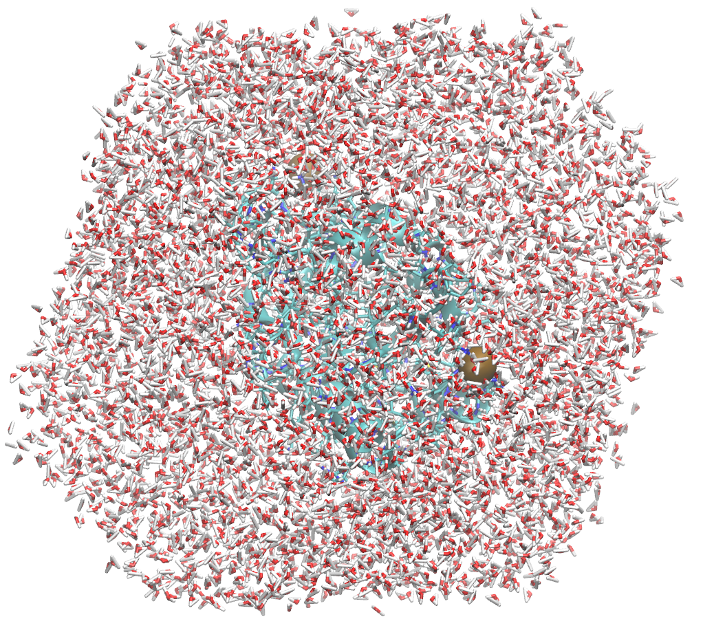
modeller = Modeller(Topology(),[])
forcefield = ForceField('amber14-all.xml', 'amber14/tip3p.xml')
modeller.addSolvent(forcefield,boxSize=(5,5,5),ionicStrength=.01*molar)
system = forcefield.createSystem(modeller.topology,  nonbondedMethod=PME,constraints=HBonds)
simulation = Simulation(modeller.topology, system, VerletIntegrator(2*femtosecond))
simulation.context.setPositions(modeller.positions)
simulation.minimizeEnergy()

show(modeller.topology, modeller.positions).show()

3Dmol.js failed to load for some reason. Please check your browser console for error messages.

Ensembles

NVE: Microcanonical

• Constant energy - no heat bath

NVT: Canonical

• This is what we've been assuming for our stat mech
• Helmholtz free energy

NPT: Isothermal-isobaric

• Changing volume makes math a bit more complicated, but pretty similar to NVT
• Gibbs free energy
• Usually most realistic

Equilibration

All simulations should start with an equilibration phase which brings the system to the target state point.

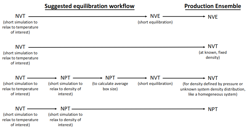
https://livecomsjournal.org/index.php/livecoms/article/view/v1i1e5957

simulation.reporters.append(StateDataReporter('output.txt', 1, step=True, volume=True,
        potentialEnergy=True, kineticEnergy=True, totalEnergy=True, temperature=True))
simulation.step(10000)

import pandas as pd
import matplotlib.pyplot as plt
data = pd.read_csv('output.txt')

data['Total Energy (kJ/mole)'].plot(); data['Potential Energy (kJ/mole)'].plot()
plt.legend(); plt.xlabel('Frame'); plt.ylabel('Energy');

data['Temperature (K)'].plot()
plt.legend(); plt.xlabel('Frame'); plt.ylabel('Temperature')

Text(0, 0.5, 'Temperature')

data['Box Volume (nm^3)'].plot()
plt.legend(); plt.xlabel('Frame');

Thermostats

We can implicitly simulate the interaction with a heat bath.

Andersen Thermostat

• Randomly select particles to experience a "collision" according to a specified collision frequency
• Set the velocity components using a Gaussian random variable $R$: $${v}_{i}=\sqrt{\frac{{k}_{B}T}{m}}R$$

system = forcefield.createSystem(modeller.topology,  nonbondedMethod=PME,constraints=HBonds)
system.addForce(AndersenThermostat(300*kelvin,1/picosecond))
simulation = Simulation(modeller.topology, system, VerletIntegrator(2*femtosecond))
simulation.context.setPositions(modeller.positions)
simulation.minimizeEnergy()
simulation.reporters.append(StateDataReporter('outputa.txt', 1, step=True, volume=True,
        potentialEnergy=True, kineticEnergy=True, totalEnergy=True, temperature=True))
simulation.step(10000)

dataa = pd.read_csv('outputa.txt')

data['Temperature (K)'].plot(label='no Thermostat')
dataa['Temperature (K)'].plot(label='w/Thermostat')
plt.legend(); plt.xlabel('Frame');

Reminder: Langevin

Uses Langevin equation of motion:

$$m_i\frac{d\mathbf{v}_i}{dt}=\mathbf{f}_i-\gamma m_i \mathbf{v}_i+\mathbf{R}_i$$

• $\mathbf{v}_i$ velocity of particle $i$
• $\mathbf{f}_i$ force acting on particle $i$
• $\mathbf{m}_i$ mass of particle $i$
• $\gamma$ friction coefficient
• $\mathbf{R}_i$ random force from normal distribution mean zero and variance $2m_i\gamma k_B T$

Integration uses Langevin leap-frog: $$\mathbf{v}_{i}(t+\Delta t/2)=\mathbf{v}_{i}(t-\Delta t/2)\alpha+\mathbf{f}_{i}(t)(1-\alpha)/\gamma{m}_{i} + \sqrt{kT(1-\alpha^2)/m}R$$ $$\mathbf{r}_{i}(t+\Delta t)=\mathbf{r}_{i}(t)+\mathbf{v}_{i}(t+\Delta t/2)\Delta t$$

$\alpha=\exp(-\gamma\Delta t)$

system = forcefield.createSystem(modeller.topology,  nonbondedMethod=PME,constraints=HBonds)
simulation = Simulation(modeller.topology, system, LangevinIntegrator(300*kelvin,1/picosecond,2*femtosecond))
simulation.context.setPositions(modeller.positions)
simulation.minimizeEnergy()
simulation.reporters.append(StateDataReporter('outputl.txt', 1, step=True, volume=True,
        potentialEnergy=True, kineticEnergy=True, totalEnergy=True, temperature=True))
simulation.step(10000)

datal = pd.read_csv('outputl.txt')

data['Temperature (K)'].plot(label='no Thermostat')
dataa['Temperature (K)'].plot(label='w/Thermostat')
datal['Temperature (K)'].plot(label='Langevin')

plt.legend(); plt.ylabel('Temperature (K)'); plt.xlabel('Frame');

%%html
<div id="energyplots" style="width: 500px"></div>
<script>
$('head').append('<link rel="stylesheet" href="https://bits.csb.pitt.edu/asker.js/themes/asker.default.css" />');

    var divid = '#energyplots';
	jQuery(divid).asker({
	    id: divid,
	    question: "What will the plots of the energy look like?",
		answers: ['KE↑,PE↑','KE↑,PE↓','KE↓,PE↑','KE↓,PE↓','Const'],
        server: "https://bits.csb.pitt.edu/asker.js/example/asker.cgi",
		charter: chartmaker})
    
$(".jp-InputArea .o:contains(html)").closest('.jp-InputArea').hide();


</script>

data['Total Energy (kJ/mole)'].plot(label='no Thermostat')
dataa['Total Energy (kJ/mole)'].plot(label='w/Thermostat')
datal['Total Energy (kJ/mole)'].plot(label='Langevin')

plt.legend(); plt.ylabel('Total Energy (kJ/mol)'); plt.xlabel('Frame');

data['Potential Energy (kJ/mole)'].plot(label='no Thermostat')
dataa['Potential Energy (kJ/mole)'].plot(label='w/Thermostat')
datal['Potential Energy (kJ/mole)'].plot(label='Langevin')

plt.legend();  plt.ylabel('Potential Energy (kJ/mol)'); plt.xlabel('Frame');

data['Kinetic Energy (kJ/mole)'].plot(label='no Thermostat')
dataa['Kinetic Energy (kJ/mole)'].plot(label='w/Thermostat')
datal['Kinetic Energy (kJ/mole)'].plot(label='Langevin')

plt.legend();  plt.ylabel('Kinetic Energy (kJ/mol)'); plt.xlabel('Frame');

Initializing Velocities

system = forcefield.createSystem(modeller.topology,  nonbondedMethod=PME,constraints=HBonds)
simulation = Simulation(modeller.topology, system, LangevinIntegrator(300*kelvin,1/picosecond,2*femtosecond))
simulation.context.setPositions(modeller.positions)
simulation.minimizeEnergy()
simulation.context.setVelocitiesToTemperature(300*kelvin) # Start at desired temperature
simulation.reporters.append(StateDataReporter('outputv.txt', 1, step=True, volume=True,
        potentialEnergy=True, kineticEnergy=True, totalEnergy=True, temperature=True))
simulation.step(10000)
datav = pd.read_csv('outputv.txt')

datal['Temperature (K)'].plot(label='Langevin')
datav['Temperature (K)'].plot(label='Langevin + Velocity Initialization')
plt.legend(); plt.ylabel('Temperature (K)'); plt.xlabel('Frame');

datal['Potential Energy (kJ/mole)'].plot(label='Langevin')
datav['Potential Energy (kJ/mole)'].plot(label='Langevin + Velocity Initialization')
plt.legend(); plt.ylabel('Potential Energy (kJ/mole)'); plt.xlabel('Frame');

Barostats

The most realistic condition for most biological systems is constant pressure/temperature (NPT: Isothermal-isobaric ensemble).

OpenMM uses a Monte Carlo barostat which periodically randomly changes the volume of the periodic box and accepts the change using the Metropolis algorithm.

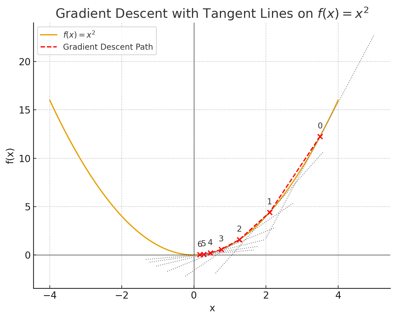
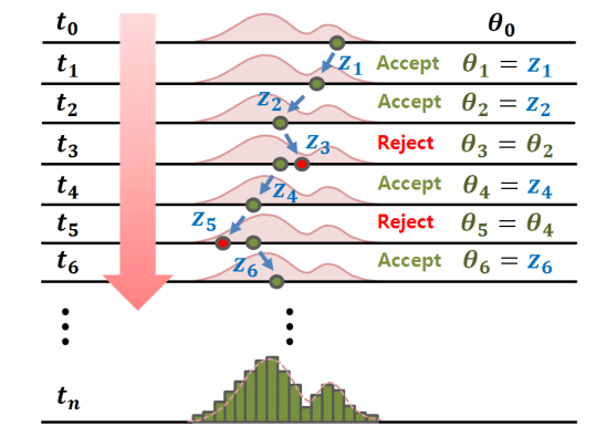
Metropolis-Hastings

The Metropolis–Hastings algorithm can draw samples from any probability distribution with probability density $P(x)$, provided that we know a function $f(x)$ proportional to the density $P$ and the values of $f(x)$ can be calculated Wikipedia.

Initialization:

• Need $g(x\mid y)$ that suggests a candidate for the next sample value $x$, given the previous sample value $y$. This is defined using a move set of perturbations you can apply to your system and might be called the proposal density or jumping distribution. Typically $g(x\mid y) = g(y\mid x)$, if not Hastings provides a correction.
• Need $f(x)$ whose value is proportional to $P(x)$
• Pick an initial configuration $x_0$

Metropolis-Hastings (continued)

For each iteration $t$:

• Generate a candidate $x'$ for the next sample by picking from the distribution $g(x'\mid x_t)$
• Calculate the acceptance ratio $\alpha = f(x')/f(x_t)$
  • $\alpha = f(x')/f(x_t) = P(x')/P(x_t)$
• Accept or reject:
  • Generate a uniform random number $u \in [0, 1]$
  • If $u \le \alpha$, then accept: $x_{t+1} = x'$
  • If $u > \alpha$, then reject: $x_{t+1} = x_t$

Why does this work?

We are essentially constructing (a very very large) Markov state model with transition probabilities $P(x'\mid x)$

If the transition probabilities fulfill detailed balance: $$P(x'\mid x)P(x) = P(x\mid x')P(x')$$

then there exists a stationary distribution $\pi$. That is, enough sampling will converge to $P(x)$.

With Metropolis, the transition probability is the product of the acceptance probability $A$ and the proposal probability $g$:

$$P(x'|x) = g(x'|x) A(x',x)$$

Plug this into the detailed balance equation and show that $$A(x', x) = \min\left(1, \frac{P(x')}{P(x)} \frac{g(x \mid x')}{g(x' \mid x)}\right)$$ fullfills detailed balance.

Detailed Balance

It states that at equilibrium, each elementary process is in equilibrium with its reverse process. Also called a reversible Markov process/chain.

$$\Large P(x) P(x \rightarrow y) = P(y) P(y \rightarrow x) \quad \forall x,y$$

Balance

A less stringent condition (does not imply reversibility).

$$\Large \sum_x P(x)P(x \rightarrow y)=p(y) \quad \forall y$$

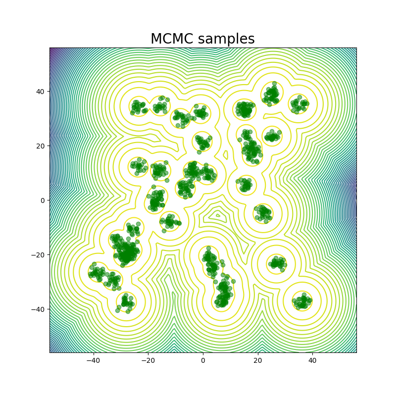
MCMC: Markov chain Monte Carlo

Metropolis-Hastings is one of a family of algorithms for stochastically sampling a probability distribution by constructing a Markov chain.

Although the algorithm produces a trajectory of states, it does not produce correct dynamics. What does this mean?

Ideally MCMC will get to equilibrium faster than traditional dynamics.

Move set can be non-physical, but must be ergodic.

Jin SS, Ju H, Jung HJ. Adaptive Markov chain Monte Carlo algorithms for Bayesian inference: recent advances and comparative study. Structure and Infrastructure Engineering. 2019 Nov 2;15(11):1548-65.

Assign2/3 Revisited

import openmm
from openmm.app import *
from openmm import *
from openmm.unit import *
import numpy as np
import matplotlib
import matplotlib.pyplot as plt
import scipy, os
import argparse
import scipy.signal

def dihedral(p1, p2, p3, p4):
    '''Return dihedral angle in radians between provided points.
    This is the same calculation used by OpenMM for force calculations. '''
    v12 = np.array(p1-p2)
    v32 = np.array(p3-p2)
    v34 = np.array(p3-p4)
    
    #compute cross products 
    cp0 = np.cross(v12,v32)
    cp1 = np.cross(v32,v34)
    
    #get angle between cross products
    dot = np.dot(cp0,cp1)
    if dot != 0:
        norm1 = np.dot(cp0,cp0)
        norm2 = np.dot(cp1,cp1)
        dot /= np.sqrt(norm1*norm2)
        
    if dot > 1.0:
        dot = 1.0
    elif dot < -1.0:
        dot = -1.0

    if dot > 0.99 or dot < -0.99:
        #close to acos singularity, so use asin isntead
        cross = np.cross(cp0,cp1)
        scale = np.dot(cp0,cp0)*np.dot(cp1,cp1)
        angle = np.arcsin(np.sqrt(np.dot(cross,cross)/scale))
        if dot < 0.0:
            angle = np.pi - angle
    else:
        angle = np.arccos(dot)
    
    #figure out sign
    sdot = np.dot(v12,cp1)
    angle *= np.sign(sdot)
    return angle
    
    
def make_rotation_matrix(p1, p2, angle):
    '''Make a rotation matrix for rotating angle radians about the p2-p1 axis'''
    # https://en.wikipedia.org/wiki/Rotation_matrix#Rotation_matrix_from_axis_and_angle
    vec = np.array((p2-p1))
    x,y,z = vec/np.linalg.norm(vec)
    cos = np.cos(angle)
    sin = np.sin(angle)
    R = np.array([[cos+x*x*(1-cos), x*y*(1-cos)-z*sin, x*z*(1-cos)+y*sin],
                  [y*x*(1-cos)+z*sin, cos+y*y*(1-cos), y*z*(1-cos)-x*sin],
                  [z*x*(1-cos)-y*sin, z*y*(1-cos)+x*sin, cos+z*z*(1-cos)]])
    return R
    
    
def moving_atoms(pdb,a=1,b=2):
    '''Identify the atoms on the b side of a dihedral with the central
    atoms a and b.  This is not the most efficient algorithm, but 
    for small molecules it really does not matter.
    A boolean mask of these atoms is returned.'''
    moving = np.zeros(pdb.topology.getNumAtoms())
    moving[b] = 1
    moving[a] = -1
    changed = True
    while changed:
        changed = False
        for b in pdb.topology.bonds():
            if (moving[b.atom1.index] + moving[b.atom2.index]) == 1:
                moving[b.atom1.index] = moving[b.atom2.index] = 1
                changed = True
    moving[1] = 0    
    return moving.astype(bool)      

# read file
pdb = PDBFile('data/gly.pdb')

# setup openmm system using amber 14 forcefield which defines the potential energy function
ff = ForceField('amber14-all.xml')
system = ff.createSystem(pdb.topology,ignoreExternalBonds=True)
# we aren't actually simulating, but need a simulation object to calculate energies
integrator = VerletIntegrator(1*femtosecond)
simulation = Simulation(pdb.topology, system, integrator)

# store atom positions
# note that more code is necessary for this code to be a general solution
# as opposed to only working with our carefully prepared inputs
origpos = np.array(pdb.getPositions()._value)
newpos = origpos.copy()

aindex, bindex = 1,2
capos = origpos[aindex]
cpos = origpos[bindex]

# a boolean mask of the atoms that should be rotated around the dihedral
mask = moving_atoms(pdb, aindex, bindex)

def get_energy(d):
    '''Return energy for amino acid at given dihedral value d (in degrees)'''
    R = make_rotation_matrix(capos,cpos,np.deg2rad(d))    
    newpos[mask] = np.matmul(R,origpos[mask].T).T     
    # setPositions to newpos in simulation 
    simulation.context.setPositions(newpos)
    # get simulation.context state, fetching energy
    state = simulation.context.getState(getEnergy=True)
    # record the energy
    return state.getPotentialEnergy()
    
energies = []
angles = []
for d in range(0,360,1):
    # record the energy
    energies.append(get_energy(d))
    # record the dihedral
    d = dihedral(*newpos[:4])
    if d < 0: d += 2*np.pi
    angles.append(np.rad2deg(d))

E = [e._value for e in energies] # unitless for numpy manipulation
T = 300*kelvin
weights = np.array([np.exp(-e/(MOLAR_GAS_CONSTANT_R*T)) for e in energies])
Z = weights.sum()
probs = weights/Z

plt.figure(figsize=(8,4),dpi=300); plt.plot(angles,probs); plt.xlabel("Dihedral (Degrees)"); plt.ylabel("Probability (at 300K)"); plt.xlim(0,360); plt.title('GLY');

Implementing MCMC

def run_mcmc(scale=360,steps=100000,T=300*kelvin,initd=0):    
    '''Return unnormalized distribution of angles from MCMC'''
    anglecnts = np.zeros(360)
    d = initd
    lastE = get_energy(d)
    lastP = np.exp(-lastE/(MOLAR_GAS_CONSTANT_R*T))
    # d is last evaluated dihedral
    for t in range(steps):    
        #propose a move
        dprime = (d + (2*np.random.random()-1)*scale)%360

        R = make_rotation_matrix(capos,cpos,np.deg2rad(dprime))    
        newpos[mask] = np.matmul(R,origpos[mask].T).T

        # setPositions to newpos in simulation 
        simulation.context.setPositions(newpos)
        state = simulation.context.getState(getEnergy=True)
        Eprime = state.getPotentialEnergy()
        Pprime = np.exp(-Eprime/(MOLAR_GAS_CONSTANT_R*T))
        # Metropolis
        if Pprime >= lastP or (np.random.random() < Pprime/lastP): # make move
            d = dprime
            anglecnts[int(np.trunc(d))] += 1
            lastP = Pprime
            lastE = Eprime
        else:
            anglecnts[int(np.trunc(d))] += 1
    return anglecnts,d

cnts, d = run_mcmc(steps=100000)
P = cnts/cnts.sum()

plt.figure(figsize=(8,4),dpi=300); plt.plot(angles,probs); plt.xlabel("Dihedral (Degrees)"); plt.ylabel("Probability (at 300K)"); plt.xlim(0,360)
plt.bar(angles,P,width=1.0,color='gold');

Effect of move set choice?

How will changing the scale factor below change how the algorithm behaves?

dprime = (d + np.random.random()*scale)%360

%%html
<div id="mcmcscale" style="width: 500px"></div>
<script>
$('head').append('<link rel="stylesheet" href="https://bits.csb.pitt.edu/asker.js/themes/asker.default.css" />');

    var divid = '#mcmcscale';
	jQuery(divid).asker({
	    id: divid,
	    question: "A smaller scale will make the convergence to the target probability distribution...",
		answers: ['Slower','Faster','Inaccurate','Nonergodic'],
        server: "https://bits.csb.pitt.edu/asker.js/example/asker.cgi",
		charter: chartmaker})
    
$(".jp-InputArea .o:contains(html)").closest('.jp-InputArea').hide();


</script>

cnts = np.zeros(360)
fig = plt.figure(figsize=(8,4)); plt.xlabel("Dihedral (Degrees)"); plt.ylabel("Probability (at 300K)"); plt.xlim(0,360); plt.plot(angles,probs); 
ax = plt.gca()
N = 20
lastd = 0
def make_fig(i):
    global cnts, lastd #the horror!
    C, lastd = run_mcmc(steps=500,initd=lastd)
    cnts += C
    P = cnts/cnts.sum()
    ax.bar(angles,P,width=1.0,color=cm.hot(i/N),alpha=.8);

anim = FuncAnimation(fig,make_fig,frames=range(N),interval=500)
video = anim.to_html5_video()
plt.close()     

html = display.HTML(video)
display.display(html)

cnts = np.zeros(360)
fig = plt.figure(figsize=(8,4)); plt.xlabel("Dihedral (Degrees)"); plt.ylabel("Probability (at 300K)"); plt.xlim(0,360); plt.plot(angles,probs); 
ax = plt.gca()
N = 20
lastd = 0
def make_fig(i):
    global cnts, lastd #the horror!
    C, lastd = run_mcmc(scale=5,steps=500,initd=lastd)
    cnts += C
    P = cnts/cnts.sum()
    ax.bar(angles,P,width=1.0,color=cm.hot(i/N),alpha=.8);

anim = FuncAnimation(fig,make_fig,frames=range(N),interval=500)
video = anim.to_html5_video()
plt.close()     

html = display.HTML(video)
display.display(html)

Metropolis algorithm step $t$ for MonteCarloBarostat

1. Generate a candidate $x'$ from distribution $g(x' | x_t)$
   • $\Delta V = A r$, $A$ is a scale factor, $r$ is a uniform random number [-1,1]
   • Box is scaled by $\Delta V$ - molecules are moved farther apart to be less dense
2. Calculate a weight function
   • $\Delta W=\Delta E+P\Delta V-Nk_{B}T \text{ln}\left(\frac{V+\Delta V}{V}\right)$
   • $\Delta E$ is change in potential energy due to box resizing
3. Accept or reject
   • If $\Delta W \le 0$
     • Leave the box resized
   • Else $\Delta W \gt 0$
     • Keep box resized with probability $e^{-\frac{\Delta W }{ k_B T}}$

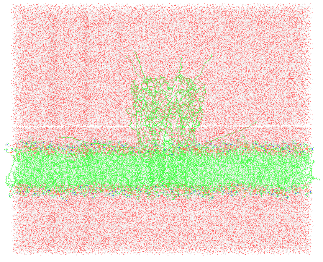
Anisotropic Barostats

When simulating a membrane typically want to keep sides of the box constant area (keep membrane in place) and so only adjust pressure at top and bottom of box.

Even better, OpenMM has a MonteCarloMembraneBarostat that includes an explicit surface tension term (S): $$\Delta W=\Delta E+P\Delta V-S\Delta A-Nk_{B}T \text{ln}\left(\frac{V+\Delta V}{V}\right)$$

system = forcefield.createSystem(modeller.topology,  nonbondedMethod=PME,constraints=HBonds)
barostat = MonteCarloBarostat(1*atmospheres, 300*kelvin, 25)
system.addForce(barostat)

simulation = Simulation(modeller.topology, system, LangevinIntegrator(300*kelvin,1/picosecond,2*femtosecond))
simulation.context.setPositions(modeller.positions)
simulation.minimizeEnergy()
simulation.reporters.append(StateDataReporter('outputp.txt', 1, step=True, volume=True,
        potentialEnergy=True, kineticEnergy=True, totalEnergy=True, temperature=True))


simulation.step(25000)

datap = pd.read_csv('outputp.txt')
datap['Box Volume (nm^3)'].plot()
plt.legend(); plt.xlabel('Frame');

MCMC Aside

A baseline for energy based models.

Analyzing MD Trajectories

https://www.mdanalysis.org/

"MDAnalysis is an object-oriented python toolkit to analyze molecular dynamics trajectories generated by CHARMM, Gromacs, NAMD, LAMMPS, or Amber."

import MDAnalysis

universe = MDAnalysis.Universe('shmtex.prmtop', 'shmtex.dcd')

MDAnalysis starts with a topology and a trajectory.

Atom Groups

universe.atoms

<AtomGroup with 85695 atoms>

You can select a specific group of atoms (very similar to pyMOL) using atom selections.

 universe.select_atoms("protein")

<AtomGroup with 14432 atoms>

Selections can work directly on AtomGroups

 universe.select_atoms("resname PRO")

<AtomGroup with 644 atoms>

 universe.select_atoms("byres around 5 resid 370")

<AtomGroup with 245 atoms>

prot = universe.select_atoms("protein")
prot.select_atoms("byres around 5 resid 370") #select whole residues within 5 of residue 100

<AtomGroup with 209 atoms>

prot.write('frame.pdb')
py3Dmol.view(data=open('frame.pdb').read(),style='cartoon:color~spectrum').show()

3Dmol.js failed to load for some reason. Please check your browser console for error messages.

Trajectories

universe.trajectory

<DCDReader shmtex.dcd with 100 frames of 85695 atoms>

The coordinates of atoms are determined by the current position in the trajectory (trajectory.frame)

The coordinates of selections refer to whatever the current trajectory frame is

The current frame is set by iterating over the trajectory or indexing into it.

for ts in universe.trajectory[:5]:
    print(ts.frame, universe.trajectory.frame, ts.time, prot.center_of_mass())

0 0 4.8888212322065376e-05 [63.06938232 61.67971211 47.8073606 ]
1 1 9.777642464413075e-05 [62.23701511 62.61718365 47.92329793]
2 2 0.00014666463696619611 [62.30295647 62.41173235 47.51776376]
3 3 0.0001955528492882615 [62.32219661 61.82873976 46.42322351]
4 4 0.0002444410616103269 [61.41691018 62.50910413 45.66813246]

Analysis

A number of packages have been contributed to MDAnalysis to perform common tasks.

import MDAnalysis.analysis

PACKAGE CONTENTS
    align - aligning structures
    contacts - native contact analysis
    density - compute water densities
    distances - for computing distances
    gnm 
    hbonds - hydrogen bond analysis
    helanal - analysis of helices
    hole - for analyzing pores
    leaflet
    nuclinfo - analysis of nucleic acids
    psa - path simularity
    rms
    waterdynamics - water analysis
    x3dna - a different nucleic analysis

MDAnalysis.rms

from MDAnalysis.analysis.rms import *  #this pulls in an rmsd function

Root mean squared deviation (RMSD) $$\sqrt{\frac{\sum_i^n(x_i^a-x_i^b)^2+(y_i^a-y_i^b)^2+(z_i^a-z_i^b)^2}{n}}$$

universe.trajectory[0] #sets the current frame to the start
refcoord = prot.positions # once stored, _coordinates_ do NOT change with trajectory
refcoord

array([[67.44726 , 79.259   , 22.918747],
       [68.181496, 78.82586 , 22.377106],
       [67.914246, 80.0178  , 23.394417],
       ...,
       [54.802658, 77.382744, 36.064526],
       [55.336662, 76.558395, 36.86686 ],
       [55.43933 , 77.794464, 35.015507]], dtype=float32)

n = universe.trajectory.n_frames
universe.trajectory[-1] #last frame
print(rmsd(refcoord,prot.positions))

38.09799719167415

protrmsd = []
carmsd = []
protref = prot.positions
caref = prot.select_atoms('name CA').positions
for ts in universe.trajectory:
    protrmsd.append(rmsd(protref,prot.positions))
    carmsd.append(rmsd(caref,prot.select_atoms('name CA').positions))

plt.plot(range(n),protrmsd,range(n),carmsd)
plt.xlabel("Frame #"); plt.ylabel('RMSD'); plt.legend(['Protein','CA'],loc='lower right');

Alignment

from MDAnalysis.analysis.align import *

Can align a single structure with alignto

Use AlignTraj to align and write out a full trajectory (trajectories are not kept in memory by default)

universe.trajectory[0]
#if we align to ourselves, will fit to current frame
alignment = AlignTraj(universe, universe, select='protein',filename='rmsfit.dcd')
alignment.run()

<MDAnalysis.analysis.align.AlignTraj at 0x72f53d9aadb0>

universe = MDAnalysis.Universe('shmtex.prmtop', 'rmsfit.dcd')
prot = universe.select_atoms('protein')

universe.trajectory[0]
protref = prot.positions
caref = prot.select_atoms('name CA').positions

protrmsd = []
carmsd = []
for ts in universe.trajectory:
    protrmsd.append(rmsd(protref,prot.positions))
    carmsd.append(rmsd(caref,prot.select_atoms('name CA').positions))

n = universe.trajectory.n_frames
plt.plot(range(n),protrmsd,range(n),carmsd)
plt.xlabel("Frame #"); plt.ylabel('RMSD'); plt.legend(['Protein','CA'],loc='lower right');

%%html
<div id="mdtri" style="width: 500px"></div>
<script>
$('head').append('<link rel="stylesheet" href="https://bits.csb.pitt.edu/asker.js/themes/asker.default.css" />');

    var divid = '#mdtri';
	jQuery(divid).asker({
	    id: divid,
	    question: "If frame 40 is ~2 RMSD from the start and frame 80 is ~2 RMSD from the start. What can be said about the RMSD between frames 40 and 80?",
		answers: ['It is ~0', 'It is < ~2','It is < ~4','Nothing'],
        server: "https://bits.csb.pitt.edu/asker.js/example/asker.cgi",
		charter: chartmaker})
    
$(".jp-InputArea .o:contains(html)").closest('.jp-InputArea').hide();


</script>

startref = prot.positions
universe.trajectory[-1]
endref = prot.positions  

startrmsd = []
endrmsd = []
for ts in universe.trajectory:
    startrmsd.append(rmsd(startref,prot.positions))
    endrmsd.append(rmsd(endref,prot.positions))

n = universe.trajectory.n_frames
plt.plot(range(n),startrmsd,range(n),endrmsd)
plt.xlabel("Frame #"); plt.ylabel('RMSD'); plt.legend(['Start RMSD','End RMSD'],loc='lower right');

RMSF

The root mean squared fluctuations of each residue/atom - the RMSD with respect to the average structure.

$$\Large \text{RMSF}_i \;=\; \sqrt{ \left\langle \big(x_i(t) - \langle x_i \rangle\big)^2 + \big(y_i(t) - \langle y_i \rangle\big)^2 + \big(z_i(t) - \langle z_i \rangle\big)^2 \right\rangle }$$

rmsf = RMSF(prot.select_atoms('name CA')).run()

plt.plot(rmsf.results.rmsf); plt.xlabel('Residue'); plt.ylabel(r'RMSF ($\AA$)');

Mapping to Structure

universe.add_TopologyAttr('tempfactors')
prot.select_atoms('name CA').tempfactors = rmsf.results.rmsf; prot.write('rmsf.pdb'); v = py3Dmol.view(data=open('rmsf.pdb').read())
v.setStyle({'cartoon':{'colorscheme':{'prop':'b','gradient':'linear','min':0,'max':5,'colors':['white','yellow','orange','red']}}}); v.show();

3Dmol.js failed to load for some reason. Please check your browser console for error messages.

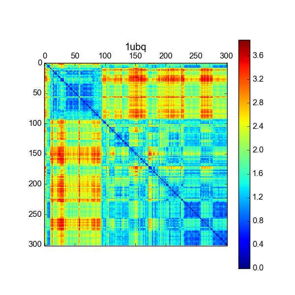
Comparative MD

Often the goal is to compare the differences in dynamics between two different starting structures, such as comparing a wild type to a disease mutant, or an bound to unbound structure.

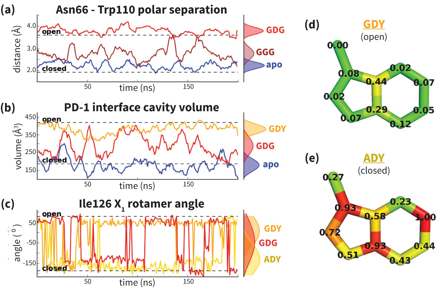
Example: Probing protein flexibility reveals a mechanism for selective promiscuity