Practical MD II

From a Simulation-Ready System to Trustworthy Results

9/23/2026

Thermodynamic state → equilibration → production → analysis → sampling

print view

%%html
<script src="https://bits.csb.pitt.edu/preamble.js"></script>
<style>:root {--jp-cell-prompt-width: 32px}</style>

Today

We already have a molecular model. Now we need to answer:

• What thermodynamic ensemble do we want?
• What happens if we simply start integrating?
• How do thermostats, velocity initialization, and barostats change the simulation?
• What does equilibrated mean in practice?
• What should we save during production?
• How do periodic boundaries and alignment affect analysis?
• How much independent information is actually in a trajectory?

Recall: System Preparation

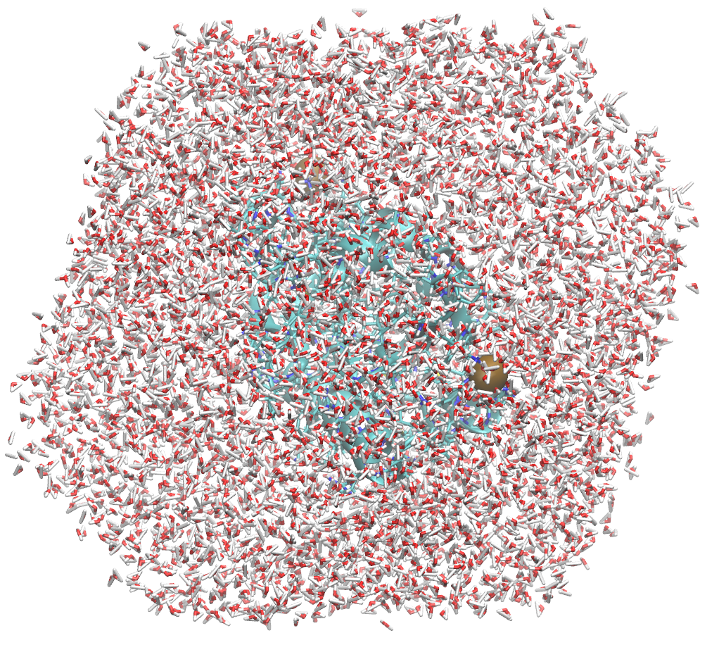
• Inspect/fix the molecular structure and chemistry
• Choose compatible protein/water/ion/ligand parameters
• Build the periodic environment with adequate padding
• Use an appropriate long-range electrostatics treatment (typically PME)
• Choose constraints and timestep
• Energy minimize and inspect

We now have a model and coordinates, but not yet an equilibrated thermodynamic ensemble.

import py3Dmol
import openmm
from openmm.app import *
from openmm.unit import *
from openmm.openmm import *

modeller = Modeller(Topology(),[])
forcefield = ForceField('amber14-all.xml', 'amber14/tip3p.xml')
modeller.addSolvent(forcefield,boxSize=(5,5,5),ionicStrength=.01*molar)
system = forcefield.createSystem(modeller.topology,  nonbondedMethod=PME,constraints=HBonds)
simulation = Simulation(modeller.topology, system, VerletIntegrator(2*femtosecond))
simulation.context.setPositions(modeller.positions)
simulation.minimizeEnergy()

show(modeller.topology, modeller.positions).show()

3Dmol.js failed to load for some reason. Please check your browser console for error messages.

What happens if we just press Run?

simulation.reporters.append(StateDataReporter('output.txt', 1, step=True, time=True,volume=True,
        potentialEnergy=True, kineticEnergy=True, totalEnergy=True, temperature=True))
simulation.step(10000)  # <--- pressing "run"

import pandas as pd
import matplotlib.pyplot as plt
data = pd.read_csv('output.txt')

data['Total Energy (kJ/mole)'].plot(); data['Potential Energy (kJ/mole)'].plot()
plt.legend(); plt.xlabel('Frame'); plt.ylabel('Energy');

data['Temperature (K)'].plot()
plt.legend(); plt.xlabel('Frame'); plt.ylabel('Temperature')

Text(0, 0.5, 'Temperature')

data['Box Volume (nm^3)'].plot()
plt.legend(); plt.xlabel('Frame');

With a Verlet integrator and no thermostat/barostat:

• Total energy should be conserved → NVE dynamics.
• Temperature is whatever follows from the kinetic energy; there is no mechanism that says “be 300 K.”
• The periodic box volume is fixed.

Minimization is not equilibration.

%%html
<div id="howlongmd" style="width: 500px"></div>
<script>
$('head').append('<link rel="stylesheet" href="https://bits.csb.pitt.edu/asker.js/themes/asker.default.css" />');

    var divid = '#howlongmd';
	jQuery(divid).asker({
	    id: divid,
	    question: "How long is our simulation?",
		answers: ['10fs','20fs','10ps','20ps','10ns','20ns'],
        server: "https://bits.csb.pitt.edu/asker.js/example/asker.cgi",
		charter: chartmaker})
    
$(".jp-InputArea .o:contains(html)").closest('.jp-InputArea').hide();


</script>

Best practice is to plot time not frames, as the meaning of a frame depends on timestep and output frequency.

Ensembles

NVE: Microcanonical

• fixed particle number, volume, and total energy
• no heat bath or pressure bath

NVT: Canonical

• fixed particle number, volume, and temperature
• natural ensemble for Helmholtz free energy

NPT: Isothermal-isobaric

• fixed particle number, pressure, and temperature; volume fluctuates
• natural ensemble for Gibbs free energy

Choose the ensemble to match the thermodynamic conditions and observable of interest. NPT is common for equilibrating condensed-phase biomolecular systems.

Thermostats

We can implicitly simulate the interaction with a heat bath.

Andersen Thermostat

• Randomly select particles to experience a "collision" according to a specified collision frequency
• Set the velocity components using a Gaussian random variable $R$: $${v}_{i}=\sqrt{\frac{{k}_{B}T}{m}}R$$

system = forcefield.createSystem(modeller.topology,  nonbondedMethod=PME,constraints=HBonds)
system.addForce(AndersenThermostat(300*kelvin,1/picosecond))
simulation = Simulation(modeller.topology, system, VerletIntegrator(2*femtosecond))
simulation.context.setPositions(modeller.positions)
simulation.minimizeEnergy()
simulation.reporters.append(StateDataReporter('outputa.txt', 1, step=True, time=True,volume=True,
        potentialEnergy=True, kineticEnergy=True, totalEnergy=True, temperature=True))
simulation.step(10000)

dataa = pd.read_csv('outputa.txt')

data['Time (ps)']

0        0.002
1        0.004
2        0.006
3        0.008
4        0.010
         ...  
9995    19.992
9996    19.994
9997    19.996
9998    19.998
9999    20.000
Name: Time (ps), Length: 10000, dtype: float64

ax=data.plot(x='Time (ps)', y='Temperature (K)', label='no Thermostat')
dataa.plot(x='Time (ps)', y='Temperature (K)', label='w/Thermostat',ax=ax)
plt.ylabel('Temperature (K)');

Reminder: Langevin

Uses Langevin equation of motion:

$$m_i\frac{d\mathbf{v}_i}{dt}=\mathbf{f}_i-\gamma m_i \mathbf{v}_i+\mathbf{R}_i$$

• $\mathbf{v}_i$ velocity of particle $i$
• $\mathbf{f}_i$ force acting on particle $i$
• $\mathbf{m}_i$ mass of particle $i$
• $\gamma$ friction coefficient
• $\mathbf{R}_i$ Gaussian random force with mean zero and variance proportional to $m_i\gamma k_B T$

Integration uses Langevin leap-frog: $$\mathbf{v}_{i}(t+\Delta t/2)=\mathbf{v}_{i}(t-\Delta t/2)\alpha+\mathbf{f}_{i}(t)(1-\alpha)/\gamma{m}_{i} + \sqrt{kT(1-\alpha^2)/m}R$$ $$\mathbf{r}_{i}(t+\Delta t)=\mathbf{r}_{i}(t)+\mathbf{v}_{i}(t+\Delta t/2)\Delta t$$

$\alpha=\exp(-\gamma\Delta t)$

system = forcefield.createSystem(modeller.topology,  nonbondedMethod=PME,constraints=HBonds)
simulation = Simulation(modeller.topology, system, LangevinIntegrator(300*kelvin,1/picosecond,2*femtosecond))
simulation.context.setPositions(modeller.positions)
simulation.minimizeEnergy()
simulation.reporters.append(StateDataReporter('outputl.txt', 1, step=True, time=True,volume=True,
        potentialEnergy=True, kineticEnergy=True, totalEnergy=True, temperature=True))
simulation.step(10000)

datal = pd.read_csv('outputl.txt')

ax=data.plot(x='Time (ps)', y='Temperature (K)', label='no Thermostat')
dataa.plot(x='Time (ps)', y='Temperature (K)', label='w/Thermostat',ax=ax)
datal.plot(x='Time (ps)', y='Temperature (K)', label='Langevin',ax=ax)
plt.ylabel('Temperature (K)');

%%html
<div id="energyplots" style="width: 500px"></div>
<script>
$('head').append('<link rel="stylesheet" href="https://bits.csb.pitt.edu/asker.js/themes/asker.default.css" />');

    var divid = '#energyplots';
	jQuery(divid).asker({
	    id: divid,
	    question: "What will the plots of the energy look like?",
		answers: ['KE↑,PE↑','KE↑,PE↓','KE↓,PE↑','KE↓,PE↓','Const'],
        server: "https://bits.csb.pitt.edu/asker.js/example/asker.cgi",
		charter: chartmaker})
    
$(".jp-InputArea .o:contains(html)").closest('.jp-InputArea').hide();


</script>

ax=data.plot(x='Time (ps)', y='Total Energy (kJ/mole)', label='no Thermostat')
dataa.plot(x='Time (ps)', y='Total Energy (kJ/mole)', label='w/Thermostat',ax=ax)
datal.plot(x='Time (ps)', y='Total Energy (kJ/mole)', label='Langevin',ax=ax)
plt.ylabel('Total Energy (kJ/mole)');

ax=data.plot(x='Time (ps)', y='Potential Energy (kJ/mole)', label='no Thermostat')
dataa.plot(x='Time (ps)', y='Potential Energy (kJ/mole)', label='w/Thermostat',ax=ax)
datal.plot(x='Time (ps)', y='Potential Energy (kJ/mole)', label='Langevin',ax=ax)
plt.ylabel('Potential Energy (kJ/mole)');

ax=data.plot(x='Time (ps)', y='Kinetic Energy (kJ/mole)', label='no Thermostat')
dataa.plot(x='Time (ps)', y='Kinetic Energy (kJ/mole)', label='w/Thermostat',ax=ax)
datal.plot(x='Time (ps)', y='Kinetic Energy (kJ/mole)', label='Langevin',ax=ax)
plt.ylabel('Kinetic Energy (kJ/mole)');

Initializing Velocities

system = forcefield.createSystem(modeller.topology,  nonbondedMethod=PME,constraints=HBonds)
simulation = Simulation(modeller.topology, system, LangevinIntegrator(300*kelvin,1/picosecond,2*femtosecond))
simulation.context.setPositions(modeller.positions)
simulation.minimizeEnergy()
simulation.context.setVelocitiesToTemperature(300*kelvin) # Start at desired temperature
simulation.reporters.append(StateDataReporter('outputv.txt', 1, step=True, time=True,volume=True,
        potentialEnergy=True, kineticEnergy=True, totalEnergy=True, temperature=True))
simulation.step(10000)
datav = pd.read_csv('outputv.txt')

ax=datal.plot(x='Time (ps)', y='Temperature (K)', label='Langevin',color='C2')
datav.plot(x='Time (ps)', y='Temperature (K)', label='Langevin + Velocity Initialization',color='C4',ax=ax)
plt.ylabel('Temperature (K)');

ax=datal.plot(x='Time (ps)', y='Potential Energy (kJ/mole)', label='Langevin',color='C2')
datav.plot(x='Time (ps)', y='Potential Energy (kJ/mole)', label='Langevin + Velocity Initialization',color='C4',ax=ax)
plt.ylabel('Potential Energy (kJ/mole)');

Thermostat practical takeaway

For most routine biomolecular work, a Langevin-family integrator is a convenient way to sample at a target temperature.

• The thermostat exchanges energy with an implicit heat bath.
• setVelocitiesToTemperature(T) avoids beginning from the artificial zero-velocity state.
  • But still need to equilibrate to get to the target temperature

The thermostat establishes temperature sampling; it does not control pressure.

Barostats

When the desired ensemble is NPT (constant pressure), the periodic box must be allowed to fluctuate.

OpenMM commonly uses a Monte Carlo barostat: it periodically proposes a box-volume change and accepts or rejects it to get the correct NPT distribution.

system = forcefield.createSystem(modeller.topology,  nonbondedMethod=PME,constraints=HBonds)
barostat = MonteCarloBarostat(1*atmospheres, 300*kelvin, 250) # this is 10X longer than the recommended default of 25
system.addForce(barostat)

simulation = Simulation(modeller.topology, system, LangevinIntegrator(300*kelvin,1/picosecond,2*femtosecond))
simulation.context.setPositions(modeller.positions); simulation.context.setVelocitiesToTemperature(300*kelvin)
simulation.minimizeEnergy()
simulation.reporters.append(StateDataReporter('outputp.txt', 1, step=True, time=True,volume=True,
        potentialEnergy=True, kineticEnergy=True, totalEnergy=True, temperature=True))


simulation.step(25000)

datap = pd.read_csv('outputp.txt')
datap.plot(x='Time (ps)', y='Box Volume (nm^3)')
plt.ylabel('Box Volume (nm^3)');

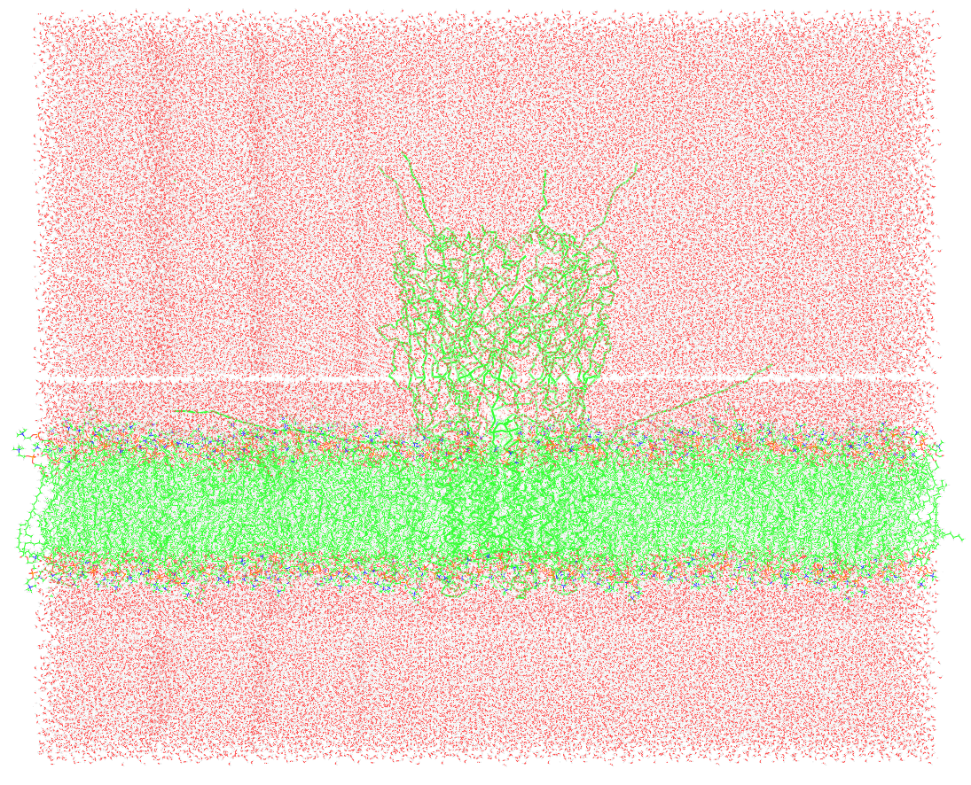
Membrane pressure coupling

Membrane simulations often use semi-isotropic pressure coupling:

• the $x$ and $y$ dimensions (membrane plane) may scale together (or not at all),
• the $z$ dimension (membrane normal) may fluctuate independently,
• a surface-tension term may be included.

OpenMM's MonteCarloMembraneBarostat supports these membrane-specific choices.

Equilibration

All simulations should start with an equilibration phase which brings the system to the target state.

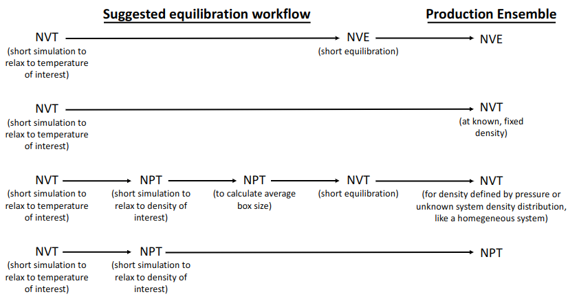
https://livecomsjournal.org/index.php/livecoms/article/view/v1i1e5957

Equilibration is observable-driven

Equilibration means allowing the artificial starting configuration to relax toward the desired state point before using the trajectory for inference.

Monitor quantities appropriate to the system:

Quantity	Why look at it?
Temperature	thermostat behaving as expected?
Potential energy	large initial relaxation finished?
Density / box volume	especially important in NPT
Structure / contacts	obvious pathology or collapse?
Restraint energy	if using staged restraints
System-specific observable	membrane area, ligand pose, pore hydration, etc.

There is no universal “X ps means equilibrated.”

Production MD

Once the system is equilibrated, run the trajectory that will actually be analyzed.

Three outputs:

1. Trajectory — coordinates for analysis
2. State log — energies, temperature, volume, etc.
3. Checkpoint/restart — enough state to continue the calculation

Do not save every 2-fs integration step just because you can: choose an output interval appropriate to the motions and analyses of interest.

# Representative production-output pattern (illustrative)
simulation.reporters.append(DCDReporter('trajectory.dcd', 5000))
simulation.reporters.append(StateDataReporter(
    'state.csv', 5000,
    step=True, time=True, potentialEnergy=True,
    temperature=True, volume=True
))
simulation.reporters.append(CheckpointReporter('checkpoint.chk', 50000))

# simulation.step(...)

A trajectory is data, not just a movie

A useful trajectory is a time-ordered set of samples from a dynamical process.

Before interpreting it, ask:

• Did the production trajectory remain consistent with the intended thermodynamic ensemble?
• Were periodic boundaries handled correctly?
• Are translation/rotation contaminating the observable?
• Is the observable relevant to the biological question?
• Are the samples sufficiently independent for the conclusion being drawn?

Analyzing MD Trajectories

Analysis workflow

$$\text{trajectory}\rightarrow\text{PBC cleanup}\rightarrow\text{alignment (when appropriate)}\rightarrow\text{observable}\rightarrow\text{statistics}$$

The preprocessing depends on the observable. For example, RMSD/RMSF usually require a whole molecule and an alignment that removes overall translation/rotation.

https://www.mdanalysis.org/

"MDAnalysis is an object-oriented python toolkit to analyze molecular dynamics trajectories generated by CHARMM, Gromacs, NAMD, LAMMPS, or Amber."

%%html
<div id="pbcq" style="width: 500px"></div>
<script>
$('head').append('<link rel="stylesheet" href="https://bits.csb.pitt.edu/asker.js/themes/asker.default.css" />');

    var divid = '#pbcq';
	jQuery(divid).asker({
	    id: divid,
	    question: "What does PBC stand for?",
		answers: ['Primary Biliary Cholangitis', 'Public Benefit Corporation','Pretty Bad Configuration','Periodic Boundary Conditions'],
        server: "https://bits.csb.pitt.edu/asker.js/example/asker.cgi",
		charter: chartmaker})
    
$(".jp-InputArea .o:contains(html)").closest('.jp-InputArea').hide();


</script>

import MDAnalysis

universe = MDAnalysis.Universe('shmtex.prmtop', 'shmtex.dcd')

MDAnalysis starts with a topology and a trajectory.

Atom Groups

universe.atoms

<AtomGroup with 85695 atoms>

You can select a specific group of atoms (very similar to pyMOL) using atom selections.

 universe.select_atoms("protein")

<AtomGroup with 14432 atoms>

Selections can work directly on AtomGroups

 universe.select_atoms("resname PRO")

<AtomGroup with 644 atoms>

 universe.select_atoms("byres around 5 resid 370")

<AtomGroup with 245 atoms>

prot = universe.select_atoms("protein")
prot.select_atoms("byres around 5 resid 370") #select whole residues within 5 of residue 370

<AtomGroup with 209 atoms>

prot.write('frame.pdb')
py3Dmol.view(data=open('frame.pdb').read(),style='cartoon:color~spectrum').show()

3Dmol.js failed to load for some reason. Please check your browser console for error messages.

Trajectories

universe.trajectory

<DCDReader shmtex.dcd with 100 frames of 85695 atoms>

The coordinates of atoms are determined by the current position in the trajectory (trajectory.frame)

The coordinates of selections refer to whatever the current trajectory frame is

The current frame is set by iterating over the trajectory or indexing into it.

for ts in universe.trajectory[:5]:
    print(ts.frame, universe.trajectory.frame, ts.time, prot.center_of_mass())

0 0 4.8888212322065376e-05 [63.06938232 61.67971211 47.8073606 ]
1 1 9.777642464413075e-05 [62.23701511 62.61718365 47.92329793]
2 2 0.00014666463696619611 [62.30295647 62.41173235 47.51776376]
3 3 0.0001955528492882615 [62.32219661 61.82873976 46.42322351]
4 4 0.0002444410616103269 [61.41691018 62.50910413 45.66813246]

Frames versus physical time

ts.frame is an index; ts.time is the physical simulation time stored/inferred for that frame (but is not always correct!).

When the x-axis represents dynamics, prefer time units such as ps or ns. Frame number is convenient bookkeeping, but its physical meaning depends on the trajectory output interval.

Analysis

A number of packages have been contributed to MDAnalysis to perform common tasks.

import MDAnalysis.analysis

PACKAGE CONTENTS
    align - aligning structures
    contacts - native contact analysis
    density - compute water densities
    distances - for computing distances
    gnm 
    hbonds - hydrogen bond analysis
    helanal - analysis of helices
    hole - for analyzing pores
    leaflet
    nuclinfo - analysis of nucleic acids
    psa - path simularity
    rms
    waterdynamics - water analysis
    x3dna - a different nucleic analysis

Analyze observables that answer the question

Start with the scientific question, then choose an observable.

Question	Analysis
Did the global structure change?	RMSD, $R_g$
Where is it flexible?	RMSF, distance/angle distributions
Did a specific interaction form?	Distances, contacts, H bonds
Which conformations are populated?	Dihedrals, distributions, clustering/PCA
Where does solvent/ion prefer to be?	Occupancy/density maps
Does one domain move relative to another?	Domain alignment + distances/angles
What are the slow collective motions?	TICA

Periodic boundaries come first

A protein can cross a periodic boundary and appear “broken” or jump across the box even though its internal structure is continuous.

Before structure-based metrics such as RMSD/RMSF, typically:

1. make molecules whole / unwrap as appropriate
2. center or re-image if useful
3. align when the observable should exclude global translation/rotation
4. compute the metric

A large raw RMSD can otherwise be a bookkeeping artifact rather than conformational change.

import MDAnalysis.transformations as trans

U = MDAnalysis.Universe('shmtex.prmtop', 'shmtex.dcd')
protein = U.select_atoms('protein')
transforms = [trans.unwrap(protein),
              trans.center_in_box(protein),
              trans.wrap(U.select_atoms('not protein'),compound='residues')]
              
U.trajectory.add_transformations(*transforms)

LOOK AT YOUR TRAJECTORY BEFORE ANALYZING

MDAnalysis.rms

from MDAnalysis.analysis.rms import *  #this pulls in an rmsd function

Root mean squared deviation (RMSD) $$\sqrt{\frac{\sum_i^n(x_i^a-x_i^b)^2+(y_i^a-y_i^b)^2+(z_i^a-z_i^b)^2}{n}}$$

universe.trajectory[0] #sets the current frame to the start
refcoord = prot.positions # once stored, _coordinates_ do NOT change with trajectory
refcoord

array([[67.44726 , 79.259   , 22.918747],
       [68.181496, 78.82586 , 22.377106],
       [67.914246, 80.0178  , 23.394417],
       ...,
       [54.802658, 77.382744, 36.064526],
       [55.336662, 76.558395, 36.86686 ],
       [55.43933 , 77.794464, 35.015507]], shape=(14432, 3), dtype=float32)

n = universe.trajectory.n_frames
universe.trajectory[-1] #last frame
print(rmsd(refcoord,prot.positions))

38.09799719167415

protrmsd = []
carmsd = []
protref = prot.positions
caref = prot.select_atoms('name CA').positions
for ts in universe.trajectory:
    protrmsd.append(rmsd(protref,prot.positions))
    carmsd.append(rmsd(caref,prot.select_atoms('name CA').positions))

plt.plot(range(n),protrmsd,range(n),carmsd)
plt.xlabel("Frame #"); plt.ylabel('RMSD'); plt.legend(['Protein','CA'],loc='lower right');

Alignment

from MDAnalysis.analysis.align import *

Can align a single structure with alignto

Use AlignTraj to align and write out a full trajectory (trajectories are not kept in memory by default)

universe.trajectory[0]
#if we align to ourselves, will fit to current frame
alignment = AlignTraj(universe, universe, select='protein',filename='rmsfit.dcd')
alignment.run()

<MDAnalysis.analysis.align.AlignTraj at 0x12ccb8590>

What should you align on?

Which atoms define the alignment?

Whole protein

• removes global translation/rotation
• useful for overall RMSD/RMSF

One domain / rigid region

• preserves motion of other regions relative to it
• useful for hinge/domain motions

What structure is the reference?

Initial structure

• measures departure from the starting conformation
• but the starting structure may be atypical

Average structure

• measures fluctuations around the mean conformation
• useful for RMSF
• align → average → realign

Experimental/reference structure

• useful when comparing to a known state

universe = MDAnalysis.Universe('shmtex.prmtop', 'rmsfit.dcd')
prot = universe.select_atoms('protein')

universe.trajectory[0]
protref = prot.positions
caref = prot.select_atoms('name CA').positions

protrmsd = []
carmsd = []
for ts in universe.trajectory:
    protrmsd.append(rmsd(protref,prot.positions))
    carmsd.append(rmsd(caref,prot.select_atoms('name CA').positions))

n = universe.trajectory.n_frames
plt.plot(range(n),protrmsd,range(n),carmsd)
plt.xlabel("Frame #"); plt.ylabel('RMSD'); plt.legend(['Protein','CA'],loc='lower right');

%%html
<div id="mdtri" style="width: 500px"></div>
<script>
$('head').append('<link rel="stylesheet" href="https://bits.csb.pitt.edu/asker.js/themes/asker.default.css" />');

    var divid = '#mdtri';
	jQuery(divid).asker({
	    id: divid,
	    question: "If frame 40 is ~2 RMSD from the start and frame 80 is ~2 RMSD from the start. What can be said about the RMSD between frames 40 and 80?",
		answers: ['It is ~0', 'It is < ~2','It is < ~4','Nothing'],
        server: "https://bits.csb.pitt.edu/asker.js/example/asker.cgi",
		charter: chartmaker})
    
$(".jp-InputArea .o:contains(html)").closest('.jp-InputArea').hide();


</script>

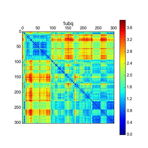
universe.trajectory[0]
startref = prot.positions
universe.trajectory[-1]
endref = prot.positions  

startrmsd = []
endrmsd = []
for ts in universe.trajectory:
    startrmsd.append(rmsd(startref,prot.positions))
    endrmsd.append(rmsd(endref,prot.positions))

n = universe.trajectory.n_frames
plt.plot(range(n),startrmsd,range(n),endrmsd)
plt.xlabel("Frame #"); plt.ylabel('RMSD'); plt.legend(['Start RMSD','End RMSD'],loc='lower right');

RMSD is not the default answer

Tokmakjian, Levon, et al. A Cationic Amphiphilic Drug (CAD) Defense System in the Nematode Caenorhabditis elegans.

Often a much simpler coordinate is more interpretable: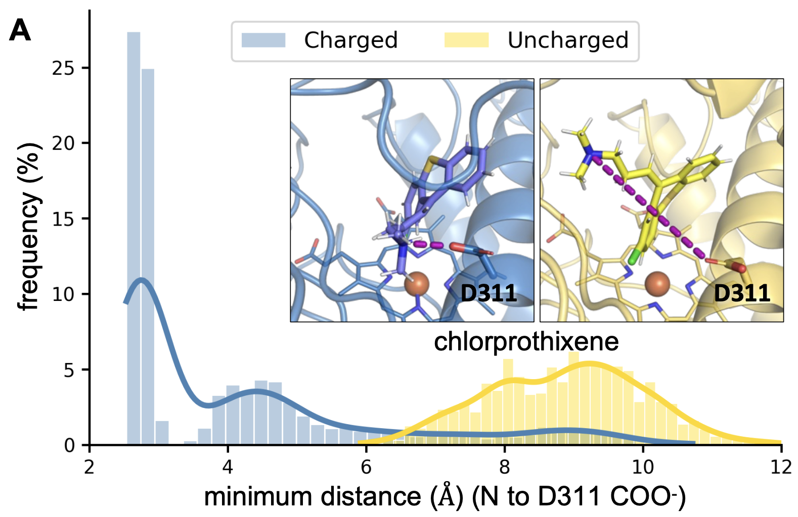

• distance between two residues/domains
• ligand–protein contact
• hydrogen-bond occupancy
• side-chain or backbone dihedral
• pore radius / ion position
• radius of gyration
• solvent occupancy

RMSF

The root mean squared fluctuations of each residue/atom - its fluctutation with respect to the average structure.

$$ \text{RMSF}_i \;=\; \sqrt{ \left\langle \big(x_i(t) - \langle x_i \rangle\big)^2 + \big(y_i(t) - \langle y_i \rangle\big)^2 + \big(z_i(t) - \langle z_i \rangle\big)^2 \right\rangle }$$

Important: Must do alignment first

ca = prot.select_atoms('name CA')
rmsf = RMSF(ca).run()

plt.plot(ca.resids, rmsf.results.rmsf); plt.xlabel('Residue'); plt.ylabel(r'RMSF ($\AA$)');

Mapping to Structure

universe.add_TopologyAttr('tempfactors')
prot.select_atoms('name CA').tempfactors = rmsf.results.rmsf; prot.write('rmsf.pdb'); v = py3Dmol.view(data=open('rmsf.pdb').read())
v.setStyle({'cartoon':{'colorscheme':{'prop':'b','gradient':'linear','min':0,'max':5,'colors':['white','yellow','orange','red']}}}); v.show();

3Dmol.js failed to load for some reason. Please check your browser console for error messages.

Comparative MD

Often the goal is to compare the differences in dynamics between two different starting structures, such as comparing a wild type to a disease mutant, or an bound to unbound structure.

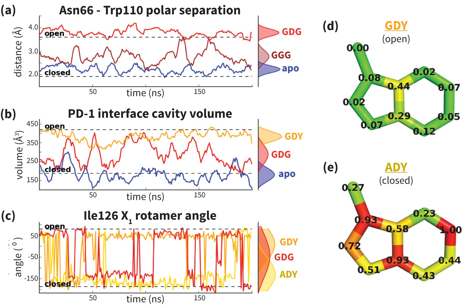
Example: Probing protein flexibility reveals a mechanism for selective promiscuity

Replicas are often more informative than one longer trajectory

Independent simulations started with different velocity seeds can reveal whether the result is robust to trajectory history.

Useful questions:

• Do independent replicas give similar distributions?
• Is one rare transition dominating an average?
• Would extending one trajectory or launching another replica teach us more?
• Are reported differences larger than simulation-to-simulation variability?

Bridge to states and kinetics

A trajectory gives us correlated configurations over time.

Next questions:

• Which configurations should be considered the same state?
• How often do we transition between states?
• How do state populations relate to thermodynamics?
• How do transition statistics give kinetics?

$$\boxed{\text{trajectory}}\rightarrow\boxed{\text{states}}\rightarrow\boxed{\text{transitions}}\rightarrow\boxed{\text{kinetics / MSMs}}$$