%%html
<script src="https://bits.csb.pitt.edu/preamble.js"></script>
<style>:root {--jp-cell-prompt-width: 32px}</style>
Quick Review
$$\Large \hat{Z}_A = \int_{x \in A} e^{\frac{-U(x)}{k_BT}}dx$$
$$\Large F_A = -k_BT\log Z_A$$
So all we have to do to get what we want is integrate...
Hopelessness
Recall 3 atom system
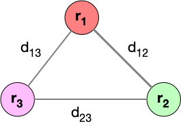
$$\Large \hat{Z} = \int \int \int e^{\frac{- \left[ u(d_{12}) + u(d_{23}) + u(d_{13}) \right]}{k_BT}}dr_1 dr_2 dr_3$$
Can't factor this.
Simulation to the Rescue!
Langevin dynamics, given long enough*, will converge to the Boltzmann distribution.
If we have enough equilibrium samples, we can compute the probability of state simply by counting how frequently it occurs!
$$\Large \int \rightarrow \sum$$
*Long enough may be really really really long...
What is a state?
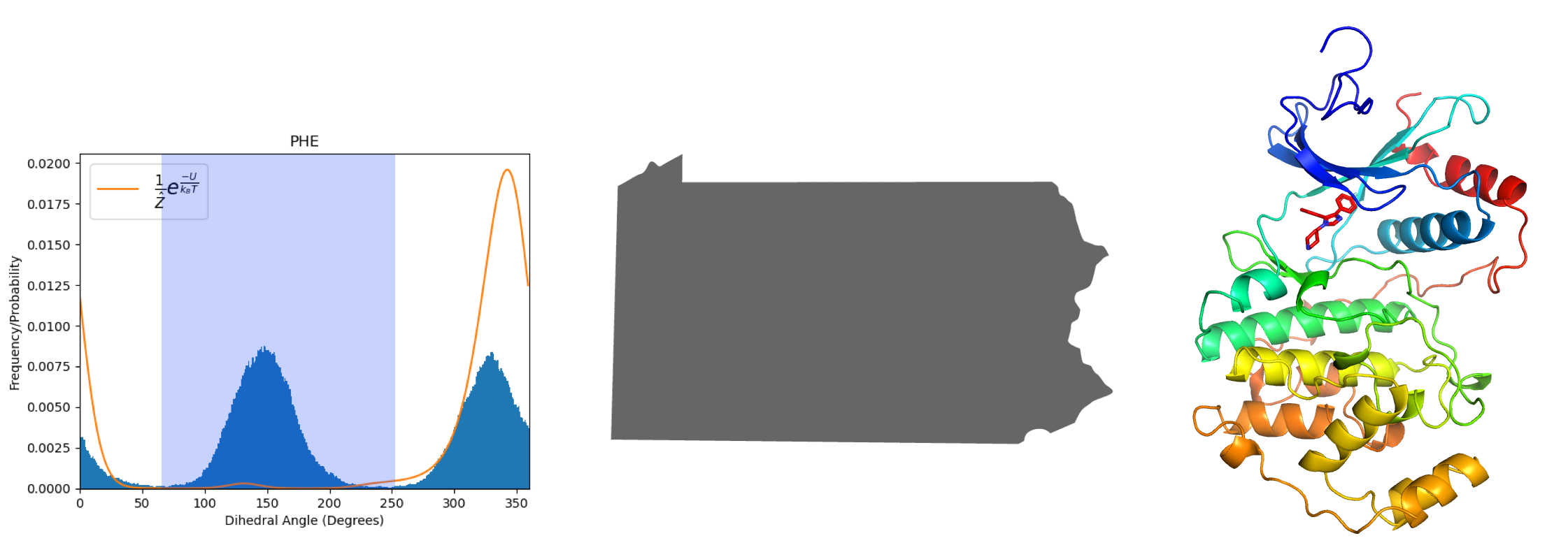
States
A state is a group of configurations (microstates).
Can define however we want, but it is desirable:
- to be around free-energy basin (high probability region)
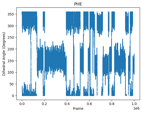
- timescales within state << timescales between states
- separation of timescales
- fast equilbration within state
- slow transitions between states
- We want Markovian dynamics - transition probabilities depend only on the current state
- separation of timescales
- states collectively partition the configuration of interest
- ideally contiguous - configuration assigned to one state form a connected region
- biological relevance
Example GPCRs
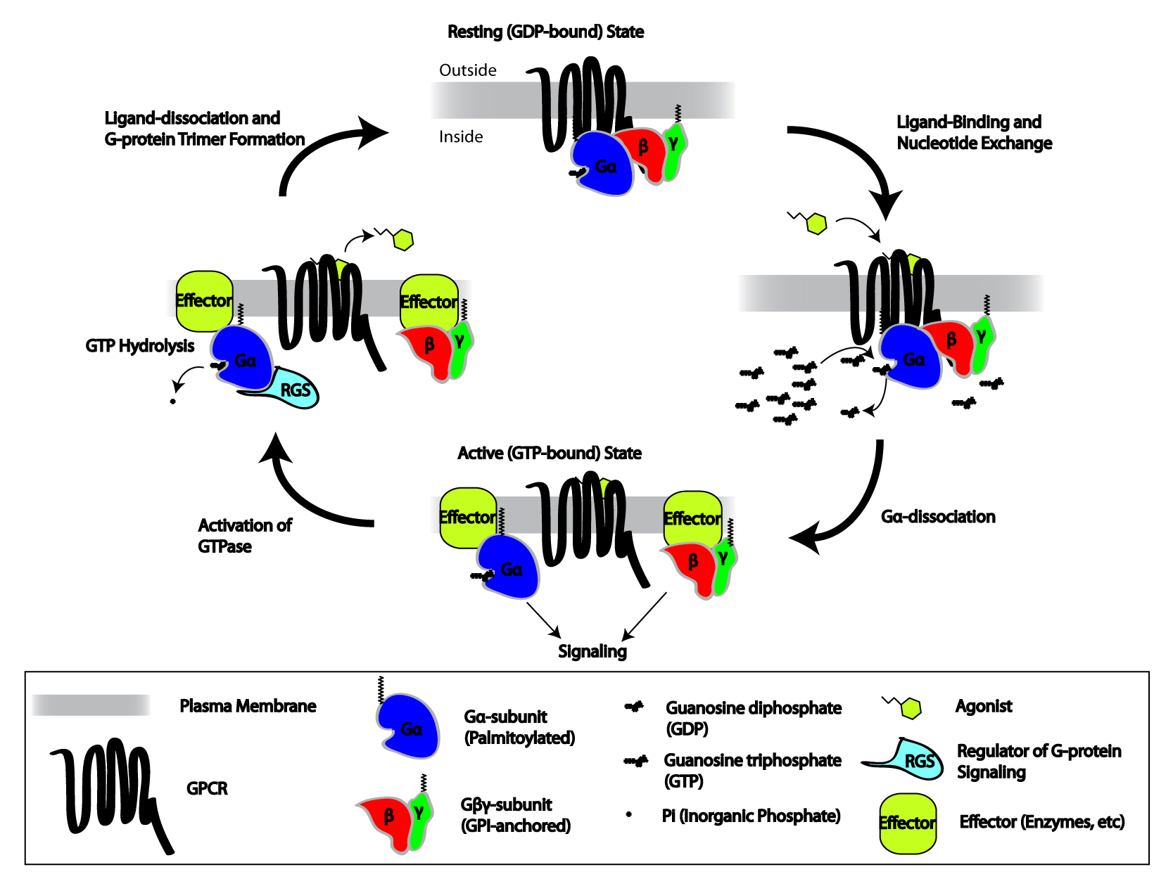
G protein-coupled receptors.
- More than 800 human GPCRs
- Membrane spanning protein that transmits signals by binding to wide variety of molecules
- proteins
- peptides
- small organic molecules
- ions
- photons (really - rhodopsin is a light sensitive GPCR in the rod cells of the retina)
- ~35% of approved drugs modulate GPCRs
https://pmc.ncbi.nlm.nih.gov/articles/PMC5820538/
| Gene Name | Example of an Approved Drug |
|---|---|
| ACKR3 | Plerixafor |
| ADGRG3 | Beclometasone dipropionate |
| ADORA1 | Adenosine |
| ADORA2A | Regadenoson |
| ADORA2B | Theophylline |
| ADORA3 | Nicardipine |
| ADRA1A | Oxymetazoline |
| ADRA1B | Prazosin |
| ADRA1D | Prazosin |
| ADRA2A | Apraclonidine |
| ADRA2B | Dexmedetomidine |
| ADRA2C | Dexmedetomidine |
| ADRB1 | Acebutolol |
| ADRB2 | Pindolol |
| ADRB3 | Mirabegron |
| AGTR1 | Candesartan |
| AVPR1A | Vasopressin |
| AVPR1B | Vasopressin |
| AVPR2 | Vasopressin |
| BDKRB1 | Icatibant |
| BDKRB2 | Icatibant |
| CALCR | Calcitonin |
| CASR | Etelcalcetide |
| CCKAR | Ceruletide |
| CCKBR | Pentagastrin |
| CCR4 | Plerixafor |
| CCR5 | Maraviroc |
| CHRM1 | Biperiden |
| CHRM2 | Propantheline |
| CHRM3 | Umeclidinium |
| CHRM4 | Acetylcholine |
| CHRM5 | Acetylcholine |
| CNR1 | Nabilone |
| CNR2 | Nabilone |
| CRHR1 | Corticorelin ovine triflutate |
| CXCR4 | Plerixafor |
| CYSLTR1 | Zafirlukast |
| CYSLTR2 | Zafirlukast |
| DRD1 | Dopamine |
| DRD2 | Dopamine |
| DRD3 | Dopamine |
| DRD4 | Dopamine |
| DRD5 | Dopamine |
| EDNRA | Ambrisentan |
| EDNRB | Bosentan |
| F2R | Vorapaxar |
| FFAR1 | Rosiglitazone |
| FPR1 | Cyclosporine |
| FSHR | Human follicle stimulating hormone |
| GABBR1 # | Baclofen |
| GABBR2 # | Baclofen |
| GCGR | Glucagon |
| GHRHR | Sermorelin |
| GLP1R | Lixisenatide |
| GLP2R | Teduglutide |
| GNRHR | Abarelix |
| GPBAR1 | Deoxycholic acid |
| GPER1 | Estradiol |
| GPR143 | Levodopa |
| GPR18 | Dronabinol |
| GPR35 | Bumetanide |
| GPR55 | Dronabinol |
| GPR68 | Lorazepam |
| HCAR1 | Sodium oxybate |
| HCAR2 | Acipimox 1 |
| HCAR3 | Nicotinic acid |
| HCRTR1 | Suvorexant |
| HCRTR2 | Suvorexant |
| HRH1 | Cetirizine |
| HRH2 | Betazole |
| HRH3 | Pitolisant * |
| HRH4 | Clozapine |
| HTR1A | Vilazodone |
| HTR1B | Frovatriptan |
| HTR1D | Frovatriptan |
| HTR1E | Asenapine |
| HTR1F | Eletriptan |
| HTR2A | Asenapine |
| HTR2B | Methysergide |
| HTR2C | Methysergide |
| HTR4 | Cisapride |
| HTR5A | Ergotamine |
| HTR6 | Amoxapine |
| HTR7 | Lurasidone |
| LHCGR | Choriogonadotropin alfa |
| MC1R | Corticotropin |
| MC2R | Corticotropin |
| MC3R | Corticotropin |
| MC4R | Corticotropin |
| MC5R | Corticotropin |
| MLNR | Erythromycin |
| MRGPRX1 | Chloroquine |
| MTNR1A | Ramelteon |
| MTNR1B | Tasimelteon |
| NPY4R | Niclosamide |
| NTSR2 | Levocabastine |
| OPRD1 | Naltrexone |
| OPRK1 | Anileridine |
| OPRM1 | Alfentanil |
| OXTR | Oxytocin |
| P2RY1 | Suramin 2 |
| P2RY11 | Suramin 2 |
| P2RY12 | Cangrelor |
| P2RY13 | Cangrelor |
| P2RY2 | Suramin 2 |
| P2RY6 | Suramin 2 |
| PTGDR | Treprostinil |
| PTGDR2 | Indomethacin |
| PTGER1 | Prostaglandin E1 |
| PTGER2 | Prostaglandin E2 |
| PTGER3 | Misoprostol |
| PTGER4 | Treprostinil |
| PTGFR | Latanoprost |
| PTGIR | Epoprostenol |
| PTH1R | Teriparatide |
| PTH2R | Teriparatide |
| S1PR1 | Fingolimod |
| S1PR2 | Fingolimod |
| S1PR3 | Fingolimod |
| S1PR4 | Fingolimod |
| S1PR5 | Fingolimod |
| SCTR | Secretin |
| SMO | Sonidegib |
| SSTR1 | Pasireotide |
| SSTR2 | Lanreotide |
| SSTR3 | Pasireotide |
| SSTR4 | Octreotide |
| SSTR5 | Lanreotide |
| SUCNR1 | Sodium succinate |
| TAAR1 | Dexamfetamine |
| TACR1 | Aprepitant |
| TBXA2R | Iloprost |
| TRHR | Protirelin |
| TSHR | Thyrotropin |

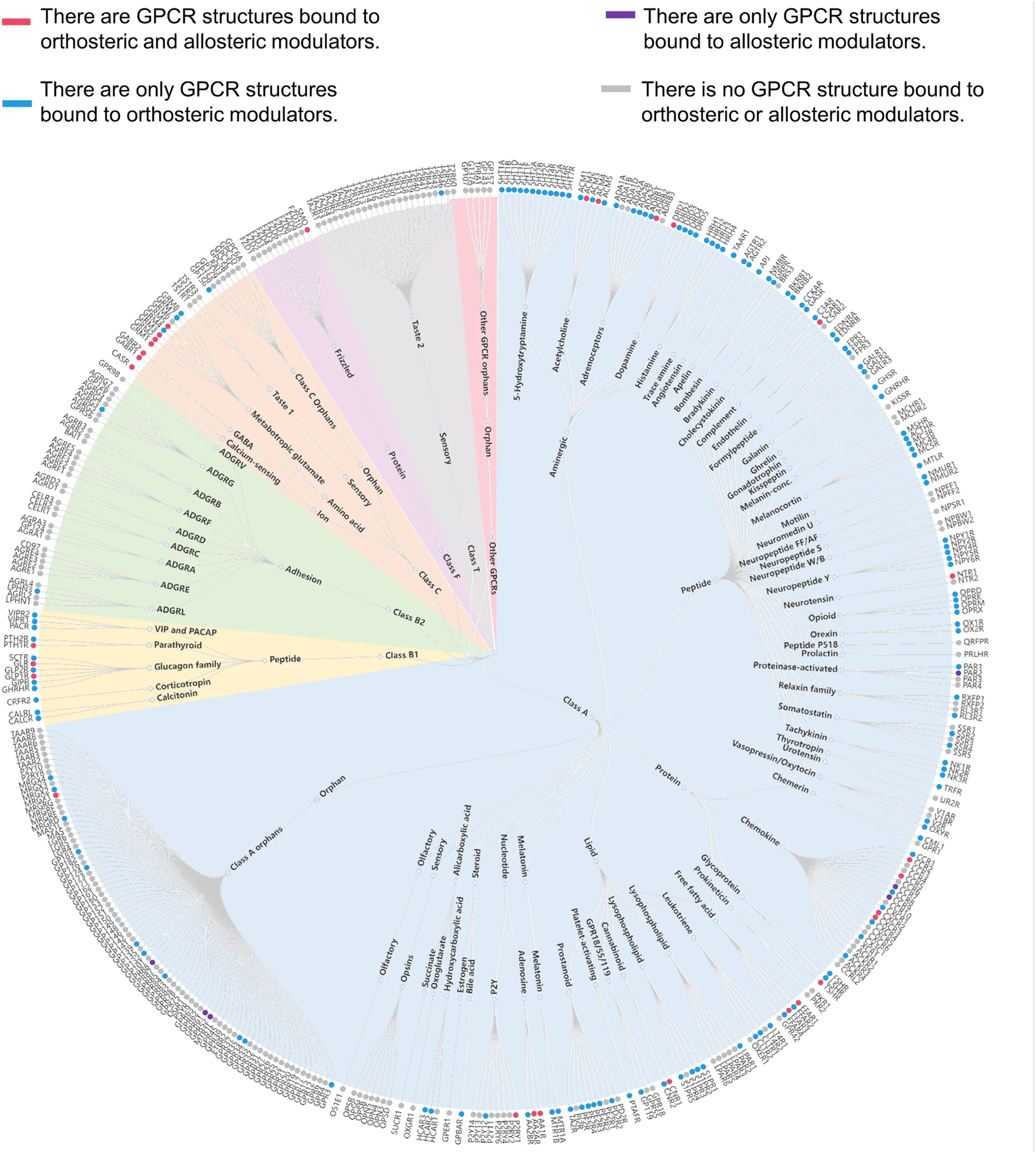
Orthosteric vs Allosteric Binding
Orthosteric ligand
Binds the receptor's native ligand-binding site.
- Competes directly with the endogenous ligand
- Often occupies the primary binding pocket
- Can act as an agonist, antagonist, or inverse agonist
Allosteric ligand
Binds at a different site on the receptor.
- Does not need to compete directly for the orthosteric site
- Changes receptor activity by altering receptor conformation
- Can enhance or inhibit the effect of the orthosteric ligand
Orthosteric = same site; allosteric = different site that modulates function
import py3Dmol; view=py3Dmol.view(query='pdb:5T1A',width=800,height=500); view.setStyle({},{'cartoon':{'color':'lightgray'}}); view.setStyle({'resi':'1002-1162'},{}); view.setStyle({'resn':'73R'},{'stick':{'colorscheme':'greenCarbon','radius':0.25}}); view.setStyle({'resn':'VT5'},{'stick':{'colorscheme':'cyanCarbon','radius':0.25}}); view.setBackgroundColor('white'); view.zoomTo({'resi':'1-1000'}); view.addLabel('Orthosteric', {'fontColor':'black','backgroundColor':'green','backgroundOpacity':0.8,'fontSize':16}, {'resn':'73R'}); view.addLabel('Allosteric', {'fontColor':'black','backgroundColor':'cyan','backgroundOpacity':0.8,'fontSize':16}, {'resn':'VT5'});view.show()
3Dmol.js failed to load for some reason. Please check your browser console for error messages.
C-C chemokine receptor 2 (CCR2) is a class A GPCR that regulates immune-cell migration and is implicated in inflammatory disease and cancer; PDB 5T1A captures CCR2 bound simultaneously to orthosteric and allosteric antagonists.
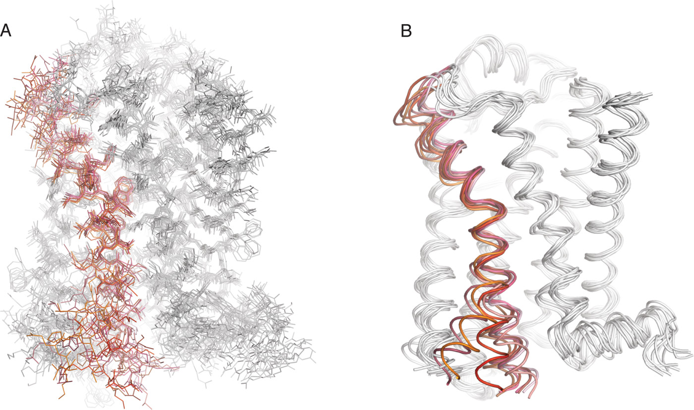
Rhodopsin
%%html
<div id="rhodstat" style="width: 500px"></div>
<script>
$('head').append('<link rel="stylesheet" href="https://bits.csb.pitt.edu/asker.js/themes/asker.default.css" />');

    var divid = '#rhodstat';
	jQuery(divid).asker({
	    id: divid,
	    question: "Which conformation is the active, signalling conformation?",
		answers: ['Blue','Tan'],
        server: "https://bits.csb.pitt.edu/asker.js/example/asker.cgi",
		charter: chartmaker})

$(".jp-InputArea .o:contains(html)").closest('.jp-InputArea').hide();


</script>
Adenosine Receptor
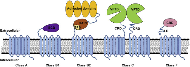
Class C GPCR (VFT domain)
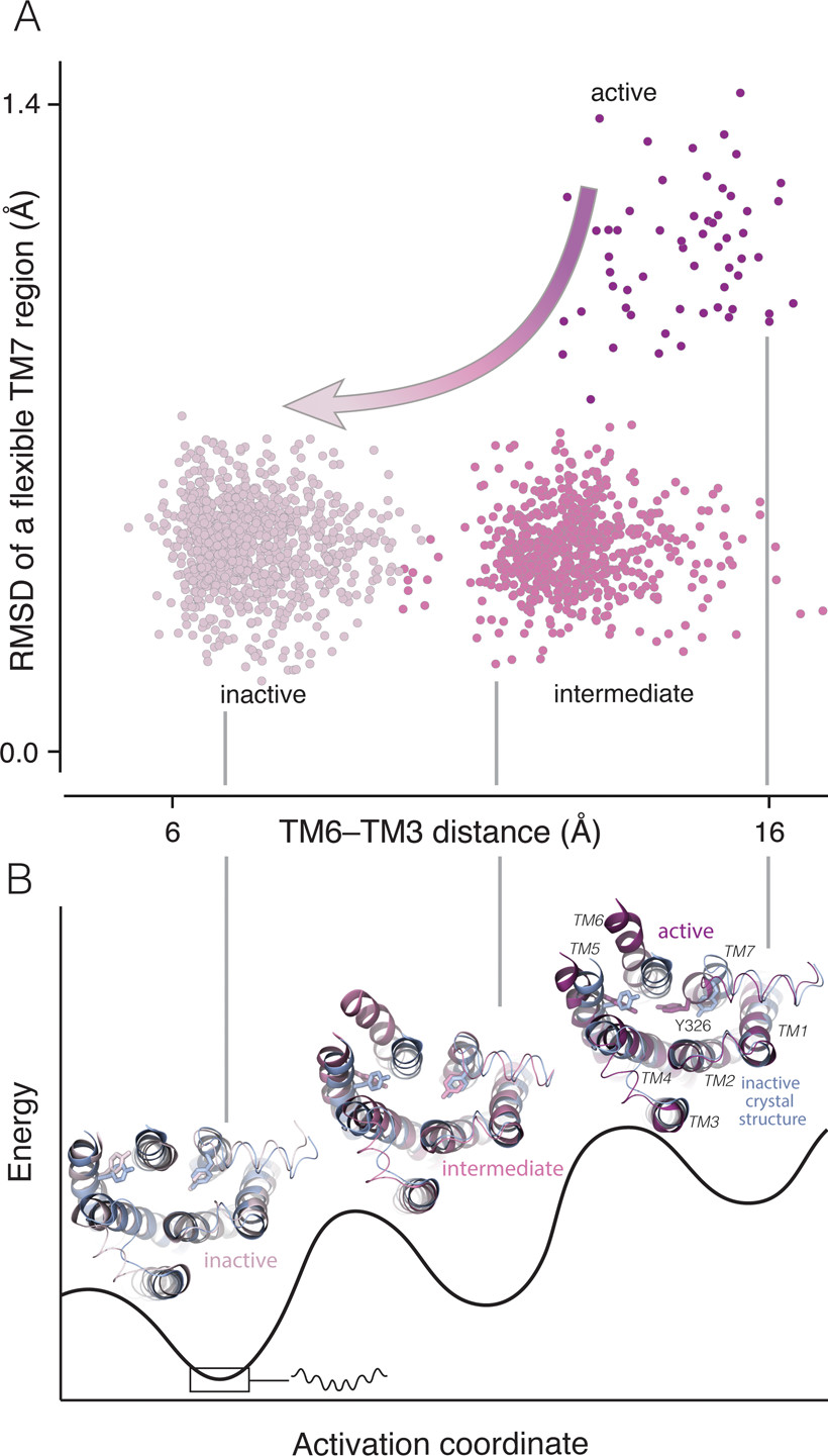
Defining States
Project to low dimensional space
- reaction or progress coordinate - typically one-dimensional
- dihedral
- distance between atoms
- distance between centers of mass
- RMSD to reference structure
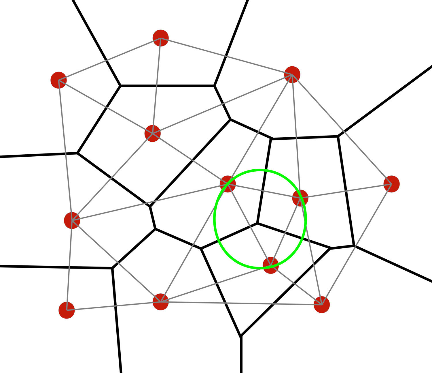 APL@Voro: A Voronoi-Based Membrane Analysis Tool for GROMACS Trajectories. https://doi.org/10.1021/ci400172g
Voronoi Tessellation
- Each state is defined by a "central" configuration
- Configurations are assigned to closest center
Potential of Mean Force
AKA, Free Energy Profile*
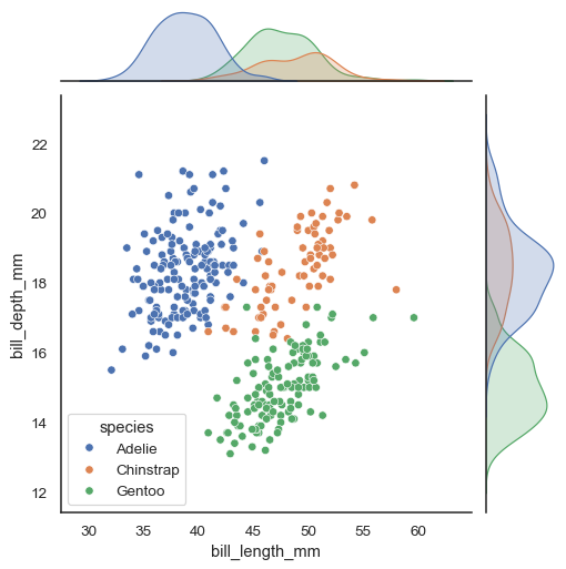
Essentially, marginalize other coordinates along reaction coordinate. "Project" onto the single coordinate of interest:
$$\rho(x) = \int \rho(x,y) dy$$ $$\rho(x) = \int \rho(x,y,z) dy dz$$
The Boltzmann factor of the PMF gives the probability distribution:
$$e^{-\mathrm{PMF}(x)/k_B T} \propto \rho(x)$$
That is,
$$\mathrm{PMF}(x) \propto -\ln \rho(x)$$
These terms are often used synonymously in the literature, but they aren't actually the same thing.
PMF General Coordinates
We have some function of coordinates, $\hat{R}(\mathbf{r}^N)$ that generates our reaction coordinate value, R (e.g. $$e^{-\mathrm{PMF}(R)/k_B T} \propto \rho(R) \propto \int \delta\left(R-\hat{R}(\mathbf{r}^N)\right) e^{-U(\mathbf{r}^N)/k_B T} d\mathbf{r}^N$$
This is a very fancy way of describing counting.
Let's calculate the PMF from assignment3
It's nothing more than the log of the normalized histogram.
import numpy as np
import matplotlib.pyplot as plt
dihedrals = np.load('dihedrals.npy')
hist,_ = np.histogram(dihedrals,bins=range(361), density=True)
PMF = -np.log(hist)
-np.log(hist) would be infinite if there are no samples. No observations does not mean infinite free energy; it means we don't have enough sampling to estimate that probability.
fig,ax = plt.subplots(figsize=(4,3),dpi=200); ax2 = ax.twinx(); xvals = np.array(range(360))+0.5; ax.plot(xvals,PMF); ax2.bar(xvals,hist,width=1,color='y',alpha=.25); ax.set_ylabel(r'$\mathrm{PMF}/k_BT$'); ax.set_xlabel("Dihedral Angle (Degrees)");ax.set_zorder(10); ax.set_frame_on(False);plt.xlim(0,360);

Why "potential of mean force"?
Free energy landscape.
This is an energy potential.
If you differentiate the potential you get the (negative) average force along the reaction coordinate (for simple coordinates, more general coordinates require geometric corrections).
But what does it all mean?
The PMF is a useful visualization. If the reaction coordinate is biophysically relevant, the transition state and barrier height may be a good approximation, but energy landscapes are complex and they could be completely wrong.
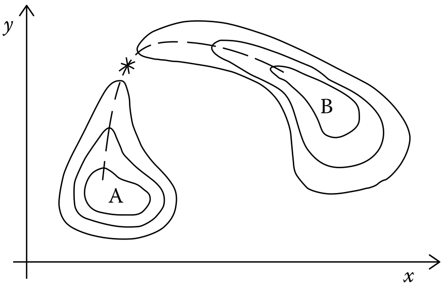
import numpy as np
import matplotlib.pyplot as plt

def multi_normal(x, mu, covariance):
    d = len(x)
    x_m = x - mu
    return ((1/(np.sqrt(2*np.pi)**d * np.linalg.det(covariance))) * np.exp(-(np.linalg.solve(covariance, x_m).T.dot(x_m))/2))[0,0]

x = np.arange(-4, 4, 0.1)
y = np.arange(-4, 4, 0.1)
xx, yy = np.meshgrid(x, y, sparse=True)
z = np.zeros((len(x), len(y)))

mean = [[-1.], [-1.]]
covariance = [
    [1., 0.8],
    [0.8, 1.]]

mean2 = [[1.], [2.]]
covariance2 = [
    [1., -0.8],
    [-0.8, 1.]]

# I DO NOT WANT TO USE THIS DOUBLE LOOP, THERE MUST BE A BETTER WAY
for i in range(len(x)):
    for j in range(len(y)):
        z[i,j] = multi_normal(np.matrix([[xx[0,i]], [yy[j,0]]]), mean, covariance)
        z[i,j] += multi_normal(np.matrix([[xx[0,i]], [yy[j,0]]]), mean2, covariance2)
fig,axes = plt.subplots(1,2,figsize=(12,4),gridspec_kw={'width_ratios': [1,2]})
h = axes[0].contourf(x,y,z)
plt.sca(axes[1])
plt.plot(x,-np.log(z.sum(axis=0)/z.sum()),label='$PMF_x/k_BT$')
plt.plot(y,-np.log(z.sum(axis=1)/z.sum()),label='$PMF_y/k_BT$')
plt.legend();

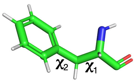

import MDAnalysis; import seaborn as sns; from MDAnalysis.analysis.dihedrals import Janin
U = MDAnalysis.Universe('phe.pdb','sim.dcd')
angles = Janin(U).run().results.angles
h = sns.jointplot(x=angles[:,0,0],y=angles[:,0,1],kind='kde',fill=True); h.set_axis_labels(r'$\chi_1$','$\chi_2$');

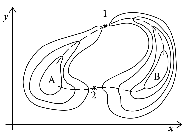
Do reaction coordinates exist?
Ideally, a "reaction coordinate" describes all essential aspects of a reaction/transformation.
In practice this may be difficult or impossible to achieve in a low dimensional space.
The Committor
An ideal reaction coordinate
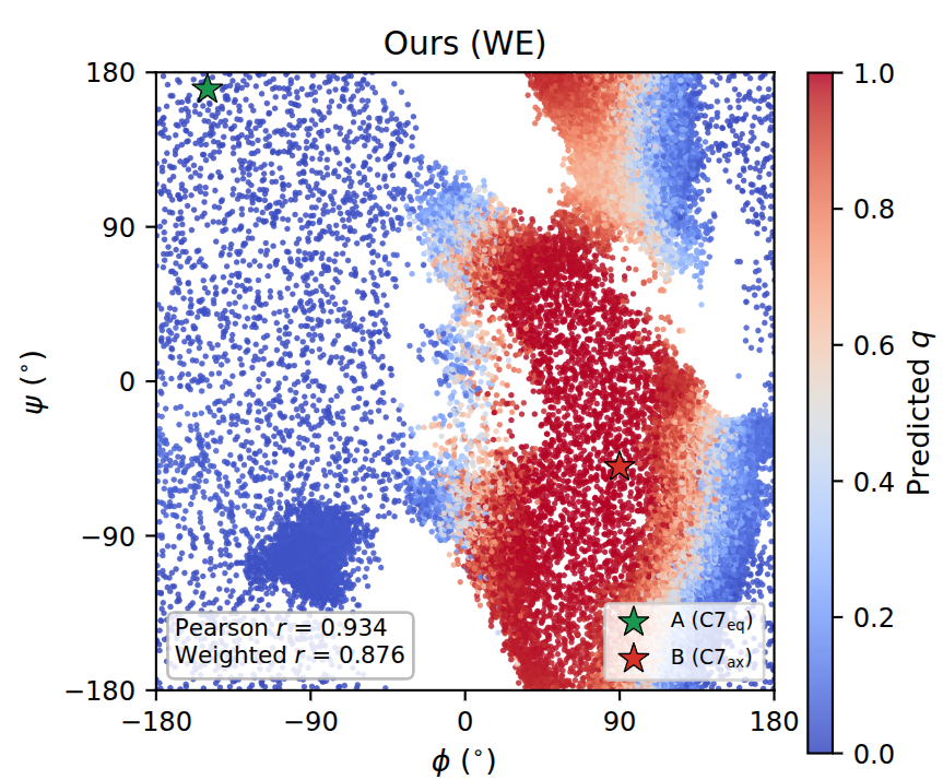
The committor gives the probability that a configuration will reach state B before state A:
$$ q(\mathbf{x}) = P(\text{reach B before A} \mid \mathbf{x}) $$
- $q(\mathbf{x}) = 0$: committed to A
- $q(\mathbf{x}) = 1$: committed to B
- $q(\mathbf{x}) = 0.5$: equally likely to reach A or B first
Configurations with $q \approx 0.5$ form the transition-state ensemble.
A good low-dimensional reaction coordinate should largely determine the committor.
But learning to estimate the committor is an active area of research and current methods essentially need to generate a full transition ensemble - which is precisely the problem we want to use the committor to solve.
Progress coordinate is a more general term - indicates progress but not necessarily the right transition path.
In practice, "reaction coordinate" tends to get used somewhat aspirationally in the literature.
Nonetheless, a good reaction coordinate can be productively used to define states.
The Kinetic Picture of States
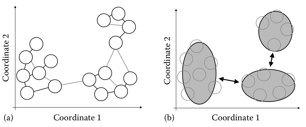
We assume that transitions between states are well described with Markovian dynamics - transitions are described by constant rates that depend only on the current state.
Basins (small circles) rapidly transition (solid lines) or slowly transition (dashed lines) leading to a coarse graining of states. Ultimately, transition probabilities come from simulation trajectories.
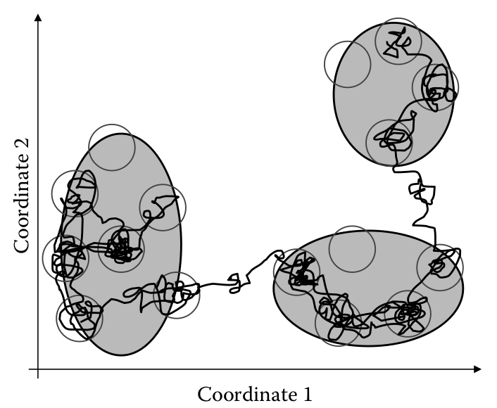
Transitions between states are dictated by fixed rates.
Warning
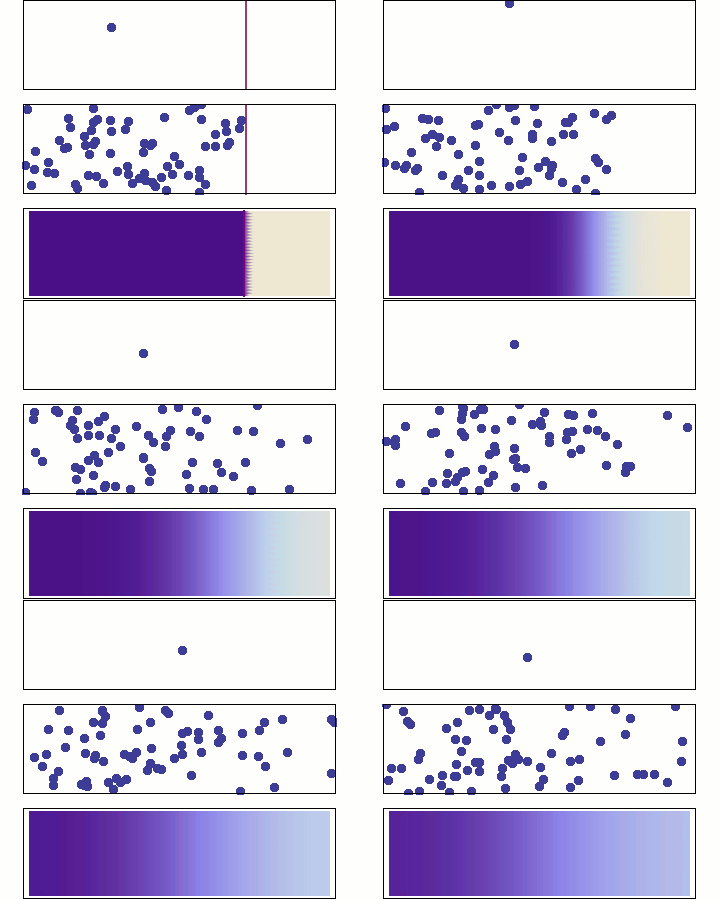
There is no guarantee that a system can be decomposed into states with separated timescales (e.g. diffusive systems).
Rates
Note: We neglect the duration of the transition path. This is reasonable when transition-path times are much shorter than residence times within states.
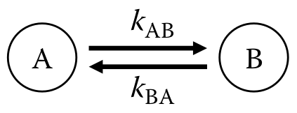
$$\Large \frac{dP_A}{dt} = k_{BA}P_B(t) - k_{AB}P_A(t)$$ $$\Large \frac{dP_B}{dt} = k_{AB}P_A(t) - k_{BA}P_B(t)$$
%%html
<div id="kunits" style="width: 500px"></div>
<script>
$('head').append('<link rel="stylesheet" href="https://bits.csb.pitt.edu/asker.js/themes/asker.default.css" />');

    var divid = '#kunits';
	jQuery(divid).asker({
	    id: divid,
	    question: "What are the units of the rate constants??",
		answers: ['None','s','1/s','M/s'],
        server: "https://bits.csb.pitt.edu/asker.js/example/asker.cgi",
		charter: chartmaker})

$(".jp-InputArea .o:contains(html)").closest('.jp-InputArea').hide();


</script>
%%html
<div id="twostatebehave" style="width: 500px"></div>
<script>
$('head').append('<link rel="stylesheet" href="https://bits.csb.pitt.edu/asker.js/themes/asker.default.css" />');

    var divid = '#twostatebehave';
	jQuery(divid).asker({
	    id: divid,
	    question: "If we start with PA(0) = 1, how will PB evolve over time?",
		answers: ['Up,flat','Up,down,flat','flat','Periodic'],
        server: "https://bits.csb.pitt.edu/asker.js/example/asker.cgi",
		charter: chartmaker})

$(".jp-InputArea .o:contains(html)").closest('.jp-InputArea').hide();


</script>
from scipy.integrate import solve_ivp
t = np.linspace(0, 10, 300)

def twostate(t, P, kAB, kBA):
    PA, PB = P
    return [kBA*PB-kAB*PA, kAB*PA-kBA*PB]

kAB = 0.5
kBA = 0.1
sol = solve_ivp(twostate, [0,10], [1,0],args=(kAB,kBA),dense_output=True)
z = sol.sol(t)
plt.plot(t, z.T)
plt.xlabel('t')
plt.legend(['$P_A$', '$P_B$'], shadow=True)
plt.show()

What happens here?
kAB = 1
kBA = 1
sol = solve_ivp(twostate, [0,10], [1,0],args=(kAB,kBA),dense_output=True)
z = sol.sol(t)
plt.plot(t, z.T)
plt.xlabel('t')
plt.legend(['$P_A$', '$P_B$'], shadow=True)
plt.show()

What about this?
kAB = .1
kBA = .9
sol = solve_ivp(twostate, [0,10], [1,0],args=(kAB,kBA),dense_output=True)
z = sol.sol(t)
plt.plot(t, z.T)
plt.xlabel('t')
plt.legend(['$P_A$', '$P_B$'], shadow=True)
plt.show()

Thermodynamics Constrains Kinetics
For
$$ A \underset{k_{BA}}{\stackrel{k_{AB}}{\rightleftharpoons}} B $$
equilibrium requires detailed balance:
$$ k_{AB}P_A^{eq} = k_{BA}P_B^{eq} \qquad\Rightarrow\qquad \frac{k_{AB}}{k_{BA}} = \frac{P_B^{eq}}{P_A^{eq}} = e^{-\beta(F_B-F_A)} = e^{-\beta\Delta F} $$
- Absolute rates determine how fast transitions occur.
- Thermodynamics constrains the ratio of forward and reverse rates.
Free energies determine equilibrium populations, not the individual rates.
The reciprocal of the rate is the average waiting time
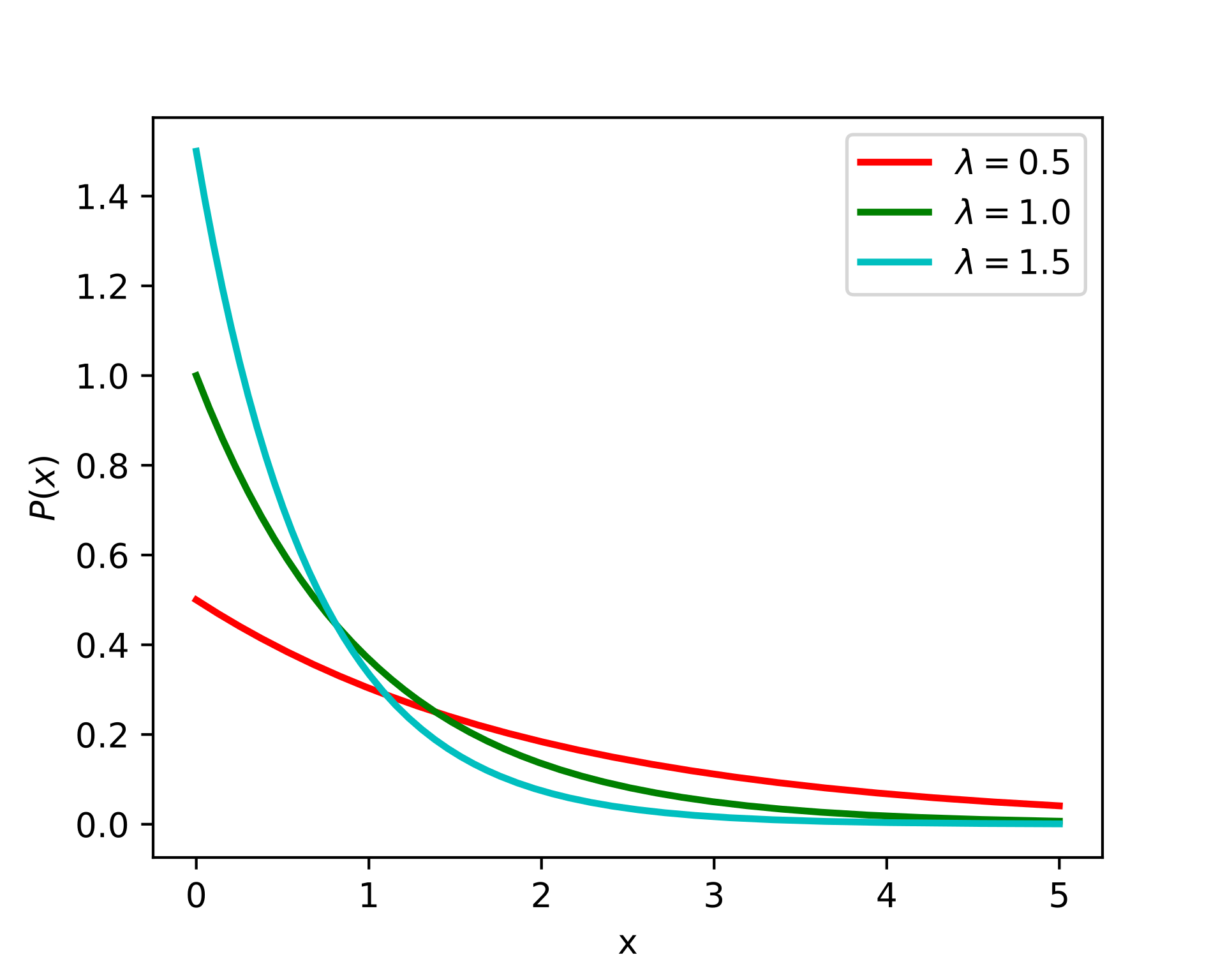
Under the Markov assumption, transitions between states are a Poisson process - "a process in which events occur continuously and independently at a constant average rate". The distribution of waiting times $t_w$ is therefore given by the exponential distribution:
$$\Large \rho(t_w) = k_{AB} \; e^{-k_{AB} t_w}$$
The mean is therefore:
$$\Large \frac{1}{k_{AB}}$$
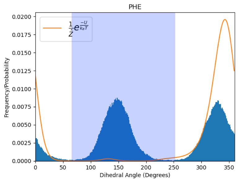
Dihedral Example
plt.figure(figsize=(4,3))
vals, _, _ = plt.hist(dihedrals,bins=range(361));

If we define State A to be between 60 and 250 degrees and state B to be everything else, what do we expect the rate constants to be?
states = (dihedrals > 60) & (dihedrals < 250) # state A is True
AB = 1
BA = 0
curr_state = states[0]
tw = 1
transition_waits = [[],[]]
for state in states[1:]:
    if state == curr_state:
        tw += 1
    else:
        transition_waits[int(curr_state)].append(tw)
        curr_state = state
        tw = 1
transition_waits[AB] = np.array(transition_waits[AB])
transition_waits[BA] = np.array(transition_waits[BA])
bins = np.linspace(0,100000,20)
plt.hist(transition_waits[AB],bins=bins,label='AB')
plt.hist(transition_waits[BA],bins=bins,alpha=.5,label='BA')
plt.legend(); plt.xlabel('Residence time'); plt.ylabel('Counts');

Mean wait time
np.mean(transition_waits[AB]),np.mean(transition_waits[BA])
(11828.39534883721, 10872.5)
Number of transitions
transition_waits[AB].shape,transition_waits[AB][transition_waits[AB] > 100].shape
((43,), (18,))
transition_waits[BA].shape,transition_waits[BA][transition_waits[BA] > 100].shape
((44,), (20,))
Beyond Two State Kinetics
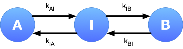
$$\begin{align} \frac{dP_A}{dt} &= -k_{AI}P_A(t) + k_{IA}P_I(t) \\ \frac{dP_I}{dt} &= k_{AI}P_A(t) - k_{IA}P_I(t) + k_{BI}P_B(t) - k_{IB}P_I(t) \\ \frac{dP_B}{dt} &= k_{IB}P_I(t) - k_{BI}P_B(t) \end{align} $$
t = np.linspace(0, 10, 300)

def threestate(t, P, kAI, kIA, kIB, kBI):
    PA, PI, PB = P
    return [-kAI*PA + kIA*PI,
            kAI*PA - kIA*PI  - kIB*PI + kBI*PB,
            kIB*PI - kBI*PB]

kAI = kIA = kIB = kBI = 0.5
sol = solve_ivp(threestate, [0,10], [1,0,0],args=(kAI,kIA, kIB, kBI),dense_output=True)
What will this look like? What will equilibrium be?
z = sol.sol(t)
plt.plot(t, z.T)
plt.xlabel('t')
plt.legend(['$P_A$', '$P_I$','$P_B$'], shadow=True)
plt.show()

What about this?
kAI = kIA = 5
kIB = kBI = .5
sol = solve_ivp(threestate, [0,10], [1,0,0],args=(kAI,kIA, kIB, kBI),dense_output=True)
z = sol.sol(t)
plt.plot(t, z.T)
plt.xlabel('t')
plt.legend(['$P_A$', '$P_I$','$P_B$'], shadow=True)
plt.show()

How about this?
kAI = kIA = 5
kIB =  0.5
kBI = 0.01
sol = solve_ivp(threestate, [0,10], [1,0,0],args=(kAI,kIA, kIB, kBI),dense_output=True)
z = sol.sol(t)
plt.plot(t, z.T)
plt.xlabel('t')
plt.legend(['$P_A$', '$P_I$','$P_B$'], shadow=True)
plt.show()

Even more rates...
With multiple states, we can define "end-to-end" rates from some initial state to some final state.
First Passage Rate: $k^{FP}$
- Inverse of mean first-passage time time (MFPT)
- Average time it takes to go from A to B
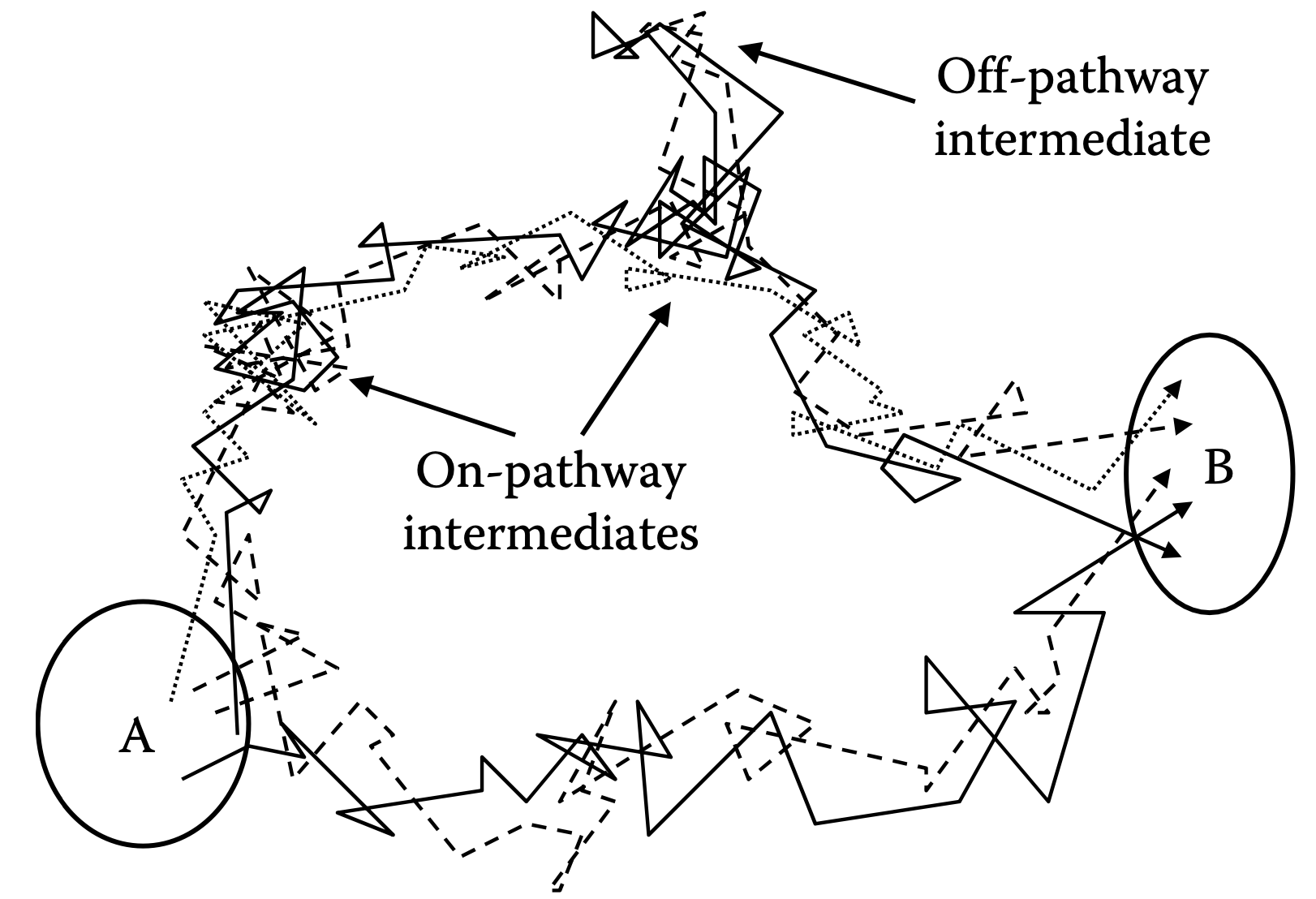
- Must consider all pathways through intermediates (e.g., AIB, AIAIB, AIAIAIB, etc..)
Steady-State Rate: $k^{SS}$
- Assumes rate of change of intermediates is zero
- All probability in B (end state) immediately transferred to A (start state)
- Things aren't changing, but not in equilibrium.
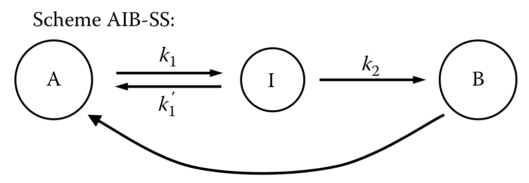
How do off pathway intermediates affect $k^{FP}$ and $k^{SS}$?