%%html
<script src="https://bits.csb.pitt.edu/preamble.js"></script>
<style>:root {--jp-cell-prompt-width: 32px}</style>
Reminder: The Kinetic Picture of States
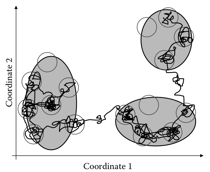
Assumption is timescale within state (how long it takes to get from one configuration to another) is much smaller than between states.
Goals of Markov State Modeling
- Describe dynamics of complex system using simple model that is
- predictive and
- interpretable
- Bridge time scales - use short trajectories to inter long time scale dynamics
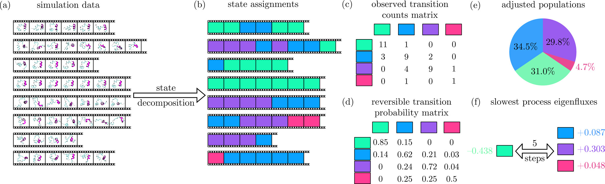

Markov process
"A stochastic model describing a sequence of possible events in which the probability of each event depends only on the state attained in the previous event."
Characterized by a transition matrix $T$:
- aka, stochastic matrix, probability matrix, substitution matrix, Markov matrix
- $T_{ij} = P(j|i)$
- $T_{ij} \ge 0$
- $\sum_j T_{ij} = 1$
An initial probability is given as a row vector, $p$, and the transition matrix is applied $pT$
Sometimes the transpose of $T$ is used, in which case: $pT = T^Tp^T$
Construct T and apply it to initial distributions...
Eigenvectors
Given a matrix $A$, a vector $\mathbf{v}$ is an eigenvector with eigenvalue $\lambda$ if it satisfies the equation: $$\Large A\mathbf{v} = \lambda\mathbf{v}$$ or, equivalently $$ (A-\lambda I)\mathbf{v} = 0 $$
Eigenvector Intuition
A matrix is a linear transformation. Eigenvectors are directions that are not changed (e.g. rotated) by this transformation. The eigenvalue is how much the transformation scales the eigenvector direction.
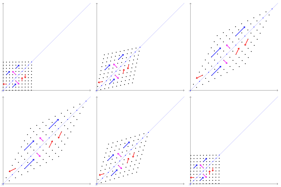
Magenta: eigenvector with eigenvalue 1
Blue: eigenvector with eigenvalue >1
Red: Not eigenvector
It is easy to solve for eigenvectors (with a computer). They are typically returned normalized to unit length.
from scipy.linalg import eig
import numpy as np
eig([[.6, .4],[.7,.3]],left=True,right=False)
(array([ 1. +0.j, -0.1+0.j]),
 array([[ 0.86824314, -0.70710678],
        [ 0.49613894,  0.70710678]]))
The left eigenvector is simply $$\Large \mathbf{v}A = \lambda\mathbf{v}$$
This is the same as the right ("normal") eigenvector of $A^T$
eig(np.array([[.6, .4],[.7,.3]]).T)
(array([ 1. +0.j, -0.1+0.j]),
 array([[ 0.86824314, -0.70710678],
        [ 0.49613894,  0.70710678]]))
What is the meaning of eigenvalue=1?
We assert without proof that, under reasonable assumptions, a transition matrix will always have an eigenvector, $\pi$, with eigenvalue 1. That is:
$$\Large \mathbf{\pi}T = \pi$$
What is the significance of $\pi$?
If all states communicate with each other, the dynamics are ergodic and there is one independent stationary distribution.
If the state space splits into disconnected components, each component has its own stationary distribution, giving multiple independent eigenvectors with $\lambda=1$.
Left and Right Eigenvectors
Our transition matrix is not generally symmetric, so it has distinct right and left eigenvectors:
$$ \Large T r_i = \lambda_i r_i $$
$$ \Large \ell_i^T T = \lambda_i \ell_i^T $$
- $r_i$: right eigenvector
- $\ell_i$: left eigenvector
- They have the same eigenvalues $\lambda_i$
A left eigenvector of $T$ is simply a right eigenvector of $T^T$.
For a reversible MSM, left and right eigenvectors describe the same dynamical modes from two perspectives: right eigenvectors assign values to states, while left eigenvectors describe how probability is distributed among those states.
Left and Right Eigenvectors for $\lambda=1$
Because $T$ is row ordered,
$$ \Large T\mathbf{1} = \mathbf{1} $$
so the right eigenvector with $\lambda=1$ is
$$ \Large r_1 = \mathbf{1}. $$
The corresponding left eigenvector satisfies
$$ \Large \pi T = \pi, $$
so
$$ \Large \ell_1 = \pi. $$
Thus:
- Right: $\mathbf{1}$ — every state has the same value
- Left: $\pi$ — the stationary probability of each state
T = np.array([[.6, .4],[.7,.3]])
pi = eig(T,left=True,right=False)[1][:,0]
pi
array([0.86824314, 0.49613894])
pi@T # @ is matrix multiplication, * is NOT
array([0.86824314, 0.49613894])
Convert to probability...
pi = pi/pi.sum()
pi
array([0.63636364, 0.36363636])
pi@T # @ is matrix multiplication, * is NOT
array([0.63636364, 0.36363636])
$\pi$ is the stationary probability
Assuming we have the correct transition probabilities, this is the Boltzmann distribution and detailed balance holds.
$$\pi_i T_{ij} = \pi_j T_{ji}$$
Since we are estimating the transition probabilities, detailed balance may not hold, but we can impose it as a constraint.
pi[0]*T[0,1]
0.2545454545454546
pi[1]*T[1,0]
0.2545454545454545
What about the second eigenvector?
ev2 = eig(T,left=True,right=False)[1][:,1]
ev2
array([-0.70710678, 0.70710678])
ev2@T
array([ 0.07071068, -0.07071068])
Backing Up: Where do states come from?
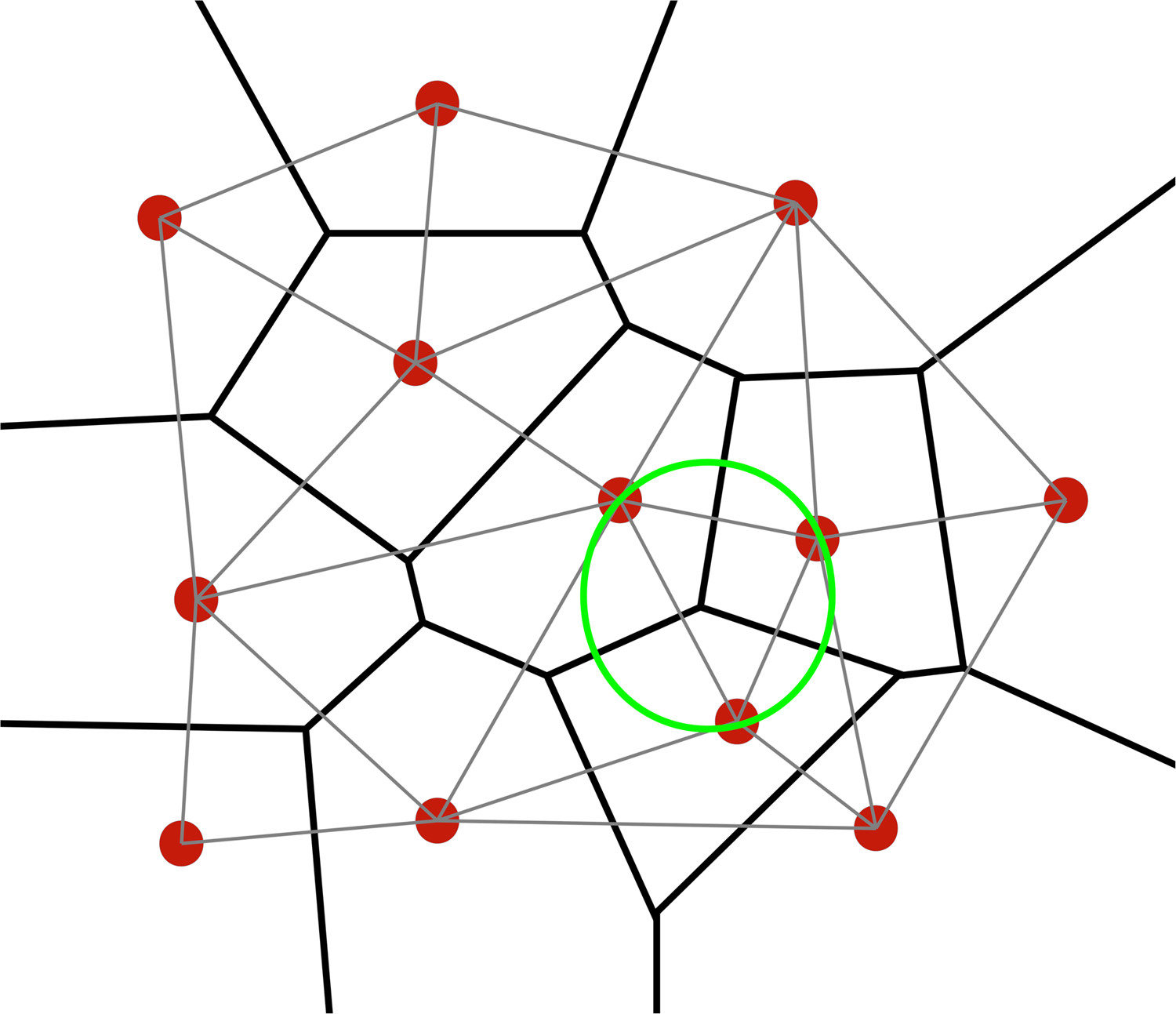 APL@Voro: A Voronoi-Based Membrane Analysis Tool for GROMACS Trajectories. https://doi.org/10.1021/ci400172g
Simplest:
- Cluster conformations from lots of simulation data
- Typically use minimal RMSD as distance metric
- What are other ways to describe conformations?
- Typically throw out water and velocities (why probably okay?)
- Define states relative to cluster center
Problems
Configurational clustering ignores kinetics.
Need a large number of small states (thousands) to (hopefully) ensure configurations in state behave kinetically similar.
But many small states means reduced sampling of transitions to/from state and bad statistics.
Solution
Cluster small states using kinetic properties into larger states.
A Running Toy Example
A single particle in a 2D double well system.
Note: We are using the legacy PyEMMA software here; deeptime is the modern, maintained, recommended MSM software).
import matplotlib.pyplot as plt
import numpy as np
import mdshare
import pyemma
pyemma.config.show_progress_bars = False

file = mdshare.fetch('hmm-doublewell-2d-100k.npz', working_directory='data')
with np.load(file) as fh:
    data = fh['trajectory']
data
array([[ 0.29565159, -0.65903237],
       [-0.32176688, -1.05838489],
       [ 0.41210344, -1.13569991],
       ...,
       [ 0.64046744, -1.62939076],
       [-0.89893827, -0.89200226],
       [ 0.77545152, -0.84004351]])
Looking at the data
plt.plot(data[:100,0],data[:100,1],c='k',lw=.5); plt.scatter(data[:100,0],data[:100,1],c=range(100));
data.shape
(100000, 2)

pyemma.plots.plot_feature_histograms(data, feature_labels=['x', 'y']);

pyemma.plots.plot_feature_histograms(data, feature_labels=['$x$', '$y$'])
for i, dim in enumerate(['y', 'x']):
    plt.plot(data[:300, 1 - i], np.linspace(-0.2 + i, 0.8 + i, 300), color='C2', alpha=0.6)
    plt.annotate('${}$(time)'.format(dim),
        xy=(3, 0.6 + i), xytext=(3, i),
        arrowprops=dict(fc='C2', ec='None', alpha=0.6, width=2))

fig, ax, misc = pyemma.plots.plot_density(data[:,0],data[:,1])
ax.set_xlabel('x'); ax.set_ylabel('y')
ax.set_xlim(-4, 4); ax.set_ylim(-4, 4); ax.set_aspect('equal')

fig, ax, misc = pyemma.plots.plot_free_energy(data[:,0],data[:,1], legacy=False)
ax.set_xlabel('x'); ax.set_ylabel('y')
ax.set_xlim(-4, 4); ax.set_ylim(-4, 4); ax.set_aspect('equal')

How is this free energy computed (from last lecture)?
States from clustering
cluster_kmeans = pyemma.coordinates.cluster_kmeans(data, k=100, stride=5,max_iter=10000)
pyemma.plots.plot_density(*data.T, cbar=False, alpha=0.1)
plt.scatter(*cluster_kmeans.clustercenters.T, s=15, c='C1')
plt.xlabel('x'); plt.ylabel('y'); plt.xlim(-4, 4); plt.ylim(-4, 4); plt.gca().set_aspect('equal')

k-means clustering
In k-means clustering we are given a set of $d$-dimensional vectors and we want to identify k sets $S_i$ such that
$$\sum_{i=1}^k \sum_{x_j \in S_i} ||x_j - \mu_i||^2$$ is minimized where $\mu_i$ is the mean of cluster $S_i$. That is, all points are close as possible to the 'center' of the cluster.
Limitations
- Classical k-means requires that we be able to take an average of our points - no arbitrary distance functions.
- Must provide $k$ as a parameter - bad $k$, bad clustering.
k-means clustering
General algorithm
- Choose initial set of $k$ cluster centers (centroids/means).
- Compute means of these clusters.
- Reassign points using updated means.
- Repeat
Will converge to local optimum.
The need for many small clusters
cluster_kmeans = pyemma.coordinates.cluster_kmeans(data, k=2, stride=5,make_iter=10000,init_strategy='uniform',fixed_seed=42)
pyemma.plots.plot_density(*data.T, cbar=False, alpha=0.1)
plt.scatter(*cluster_kmeans.clustercenters.T, s=15, c='C1')
plt.xlabel('x'); plt.ylabel('y'); plt.xlim(-4, 4); plt.ylim(-4, 4); plt.gca().set_aspect('equal')

c = pyemma.coordinates.assign_to_centers(data,cluster_kmeans.clustercenters)
plt.scatter(*data.T, c=c,marker='.')
plt.xlabel('x'); plt.ylabel('y'); plt.xlim(-4, 4); plt.ylim(-4, 4); plt.gca().set_aspect('equal');

Dimensionality Reduction
Simulation trajectories are large. It is desirable to reduce their dimensionality
- To speed things up (cluster using reduced coordinates)
- To ideally identify more relevant coordinates
Principal Components Analysis
Principal component analysis (PCA) is a statistical procedure that uses an orthogonal transformation to convert a set of observations of possibly correlated variables into a set of values of linearly uncorrelated variables called principal components. The number of principal components is less than or equal to the number of original variables. This transformation is defined in such a way that the first principal component has the largest possible variance (that is, accounts for as much of the variability in the data as possible), and each succeeding component in turn has the highest variance possible under the constraint that it is orthogonal to the preceding components. The resulting vectors are an uncorrelated orthogonal basis set. --Wikipedia

PCA
The principal components are the eigenvectors of the covariance matrix of the centered coordinates.
We are subtracting the mean coordinates for the whole trajectory from each timestep $$\tilde{\mathbf{x}}(t) = \mathbf{x}(t)-\pmb{\mu}$$
Compute the covariance matrix $C$, where $$C_{ij} = \langle \tilde{x}_i(t)\tilde{x}_j(t) \rangle_t$$
Solve for eigenvalues/vectors
$$C\mathbf{u}_i = \lambda_i\mathbf{u}_i$$
PCA Properties

If we choose the first $m$ eigenvectors to get $$\mathbf{U} = [\mathbf{u}_1,\dots,\mathbf{u}_m]$$
then the transformed (lower dimension) coordinates $\mathbf{y}$ are $$\mathbf{y}(t) = \mathbf{U}^T\tilde{\mathbf{x}}(t)$$
Let $\lambda_i \rightarrow \sigma^2_i$ to emphasize the eigenvalues measure the variance of the data along the principal direction (eigenvectors):
$$ \langle y_i(t)^2 \rangle_t = \sigma^2_i$$
The PCA basis is orthogonal, so new coordinates are uncorrelated: $$\langle y_i(t)y_j(t)\rangle = 0$$
PCA on Toy Example
What will it look like?
pyemma.plots.plot_density(*data.T, cbar=False, alpha=0.1)
plt.xlabel('x'); plt.ylabel('y'); plt.xlim(-4, 4); plt.ylim(-4, 4); plt.gca().set_aspect('equal')

pca = pyemma.coordinates.pca(data, dim=1)
pca_output = pca.get_output()
pca_output # the transformed coords
[array([[-0.26751208],
        [ 0.37113857],
        [-0.35730326],
        ...,
        [-0.55788803],
        [ 0.9381754 ],
        [-0.73651516]], dtype=float32)]
fig, axes = plt.subplots(1, 2, figsize=(10, 4))
pyemma.plots.plot_feature_histograms( np.concatenate([pca_output[0]], axis=1), feature_labels=['PCA'],  ax=axes[0])
pyemma.plots.plot_density(*data.T, ax=axes[1], cbar=False, alpha=0.1)
axes[1].plot([0, 3 * pca.eigenvectors[0, 0]], [0, 3 * pca.eigenvectors[1, 0]],  linewidth=3,   label='PCA'); axes[1].set_ylim(-4,4); axes[1].set_xlim(-4,4);

Time-lagged Independent Component Analysis (TICA)
PCA doesn't care about time, but what we are most interested in is separating time scales. Can we project onto a lower dimensional space that does this?
Yes - instead of maximizing variance (PCA), let's maximize autocorrelation at some time lag $\tau$.
Construct the time-lagged covariance matrix $C(\tau)$, where
$$c_{ij}(\tau) = \langle \tilde{x}_i(t) \tilde{x}_j(t+\tau) \rangle_t$$
Now solve for eigenvalues/vectors using this equation:
$$C(\tau)\mathbf{u}_i = C(0) \lambda_i(\tau)\mathbf{u}_i$$
What's $C(0)$?
Detail: Need to symmetrize $C(\tau)$ by averaging it with its transpose.
TICA Properties
If we choose the first $m$ eigenvectors to get
$$ \mathbf{U} = [\mathbf{u}_1,\dots,\mathbf{u}_m] $$
then the transformed (lower dimensional) coordinates $\mathbf{y}$ are
$$ \mathbf{y}(t) = \mathbf{U}^T\tilde{\mathbf{x}}(t) $$
The TICA coordinates are normalized to have unit variance and are uncorrelated with each other:
$$ \left\langle y_i(t)^2 \right\rangle = 1 $$
$$ \left\langle y_i(t)y_j(t) \right\rangle = 0 \qquad i\neq j $$
At the lag time $\tau$, each coordinate is correlated with itself according to its eigenvalue:
$$ \left\langle y_i(t)y_i(t+\tau) \right\rangle = \lambda_i $$
while different TICA coordinates remain uncorrelated:
$$ \left\langle y_i(t)y_j(t+\tau) \right\rangle = 0 \qquad i\neq j $$
Thus, large $\lambda_i$ means that $y_i$ changes slowly and represents a slow dynamical process.
TICA on Toy Example
tica = pyemma.coordinates.tica(data, dim=1, lag=1)
tica_output = tica.get_output()
tica_output
[array([[-0.42423657],
        [-0.73914737],
        [-0.79901934],
        ...,
        [-1.1870486 ],
        [-0.6090164 ],
        [-0.5659988 ]], dtype=float32)]
fig, axes = plt.subplots(1, 2, figsize=(10, 4))
pyemma.plots.plot_feature_histograms( np.concatenate([pca_output[0], tica_output[0]], axis=1),feature_labels=['PCA', 'TICA'],    ax=axes[0])
pyemma.plots.plot_density(*data.T, ax=axes[1], cbar=False, alpha=0.1)
axes[1].plot( [0, 3 * pca.eigenvectors[0, 0]],    [0, 3 * pca.eigenvectors[1, 0]],    linewidth=3,    label='PCA')
axes[1].plot( [0, 3 * tica.eigenvectors[0, 0]],    [0, 3 * tica.eigenvectors[1, 0]], linewidth=3,  label='TICA')
axes[1].set_xlabel('$x$'); axes[1].set_ylabel('$y$'); axes[1].set_xlim(-4, 4); axes[1].set_ylim(-4, 4);axes[1].set_aspect('equal'); axes[1].legend();

cluster_kmeans = pyemma.coordinates.cluster_kmeans(tica_output, k=2, stride=5,max_iter=10000,init_strategy='uniform',fixed_seed=42)
c = pyemma.coordinates.assign_to_centers(tica_output,cluster_kmeans.clustercenters)
plt.scatter(*data.T, c=c,marker='.')
plt.scatter([0,0],cluster_kmeans.clustercenters.T, s=15, c='C1')
plt.xlabel('x'); plt.ylabel('y'); plt.xlim(-4, 4); plt.ylim(-4, 4); plt.gca().set_aspect('equal');

cluster_kmeans.clustercenters
array([[ 0.8785797],
       [-0.6902315]], dtype=float32)
From States to Transition Matrix
For a given lag time $\tau$ we have a count matrix $\mathrm{C}$ where $\mathrm{c}_{ij}$ is simply the number of times in our simulation data we have seen a configuration in state $i$ at time $t$ transition to state $j$ at time $t+\tau$.
We want the most likely Markov transition matrix $T$.
We assert without proof that this is given by:
$$\mathrm{t}_{ij} = \frac{\mathrm{c}_{ij}}{\sum_k c_{ik}}$$
Note that if we want to additionally impose the constraint that $T$ obeys detailed balance, the math gets more complicated.
Eigenvectors of the Transition Matrix
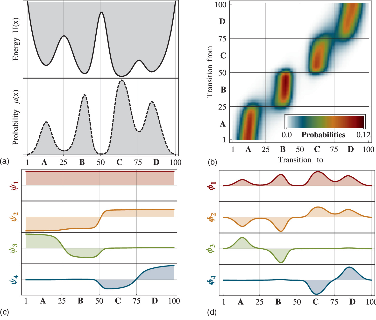
Prinz JH, Wu H, Sarich M, Keller B, Senne M, Held M, Chodera JD, Schütte C, Noé F. Markov models of molecular kinetics: Generation and validation. The Journal of chemical physics. 2011 May 7;134(17):174105.
How good is our model?
The transition matrix $T$ is basically the model, but does it represent the dynamics we are interested in?
Let $p(t)$ be the probability distribution of states at time $t$, how good is the approximation:
$$p(n\tau) \approx p(0)T^n(\tau)$$
A good indicator (but not guarantee) that $\tau$ is in the right range is that the implied timescales stay constant.
What is an Implied Timescale?
Each eigenvalue describes how quickly a dynamical mode decays.
After one lag time $\tau$:
$$ \text{mode amplitude} \rightarrow \lambda_i(\tau)\times\text{mode amplitude} $$
After $n$ lag times:
$$ \text{mode amplitude} \rightarrow \lambda_i(\tau)^n $$
A relaxation process with timescale $t_i$ decays exponentially:
$$ e^{-t/t_i} $$
Setting $t=n\tau$ gives
$$ \lambda_i(\tau)^n = e^{-n\tau/t_i} $$
and therefore
$$ \boxed{ t_i(\tau)=-\frac{\tau}{\ln|\lambda_i(\tau)|} } $$
This is the implied timescale: the relaxation time implied by an MSM constructed at lag time $\tau$.
Toy Example
cluster = pyemma.coordinates.cluster_kmeans(data, k=2, stride=5,make_iter=10000,init_strategy='uniform',fixed_seed=42)
pyemma.plots.plot_density(*data.T, cbar=False, alpha=0.1)
plt.scatter(*cluster.clustercenters.T, s=15, c='C1')
plt.xlabel('x'); plt.ylabel('y'); plt.xlim(-4, 4); plt.ylim(-4, 4); plt.gca().set_aspect('equal');
cluster.dtrajs[0]
array([1, 1, 1, ..., 1, 0, 1], dtype=int32)
its = pyemma.msm.its(cluster.dtrajs, lags=[1, 2, 3, 5, 7, 10], nits=1,n_jobs=1)
pyemma.plots.plot_implied_timescales(its, ylog=False);

cluster = pyemma.coordinates.cluster_kmeans(data, k=3, max_iter=500)
pyemma.plots.plot_density(*data.T, cbar=False, alpha=0.1)
plt.scatter(*cluster.clustercenters.T, s=15, c='C1')
plt.xlabel('x'); plt.ylabel('y'); plt.xlim(-4, 4); plt.ylim(-4, 4); plt.gca().set_aspect('equal');

its = pyemma.msm.its(cluster.dtrajs, lags=[1, 2, 3, 5, 7, 10], nits=2,n_jobs=1)
pyemma.plots.plot_implied_timescales(its, ylog=False);

cluster = pyemma.coordinates.cluster_kmeans(data, k=50, max_iter=500)
pyemma.plots.plot_density(*data.T, cbar=False, alpha=0.1)
plt.scatter(*cluster.clustercenters.T, s=15, c='C1')
plt.xlabel('x'); plt.ylabel('y')
plt.xlim(-4, 4); plt.ylim(-4, 4); plt.gca().set_aspect('equal');

its = pyemma.msm.its(cluster.dtrajs, lags=[1, 2, 3, 5, 7, 10],n_jobs=1)
pyemma.plots.plot_implied_timescales(its, ylog=False);

There's only one "thing" happening with a timescale longer than the lag time.
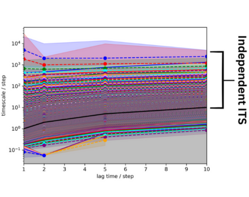
MSM Analysis
msm = pyemma.msm.estimate_markov_model(cluster.dtrajs, lag=1)
msm.stationary_distribution
array([0.01463015, 0.0224302 , 0.01337016, 0.02845033, 0.0196402 ,
       0.00710003, 0.03010025, 0.02628029, 0.01534014, 0.01395012,
       0.03285025, 0.01018012, 0.02035023, 0.00884009, 0.01908022,
       0.03312038, 0.0184602 , 0.0402804 , 0.02539023, 0.0180502 ,
       0.00433005, 0.02606029, 0.02071017, 0.02143019, 0.02644035,
       0.01045012, 0.00589007, 0.02012024, 0.01146007, 0.02141025,
       0.01971022, 0.02464026, 0.02222015, 0.01834019, 0.02144023,
       0.01173012, 0.00433002, 0.03698038, 0.01649015, 0.03289036,
       0.01893015, 0.02304017, 0.02241024, 0.01249014, 0.03208029,
       0.0121501 , 0.01488018, 0.03304028, 0.01369015, 0.02232025])
fig, ax, misc = pyemma.plots.plot_contour(  *data.T, msm.pi[cluster.dtrajs[0]],   cbar_label='stationary distribution',    method='nearest', mask=True)
ax.scatter(*cluster.clustercenters.T, s=15, c='C1')
ax.set_xlabel('$x$');ax.set_ylabel('$y$')
ax.set_xlim(-4, 4);ax.set_ylim(-4, 4);ax.set_aspect('equal')

Contrast with data density...
fig, ax, misc = pyemma.plots.plot_density(data[:,0],data[:,1])
ax.set_xlabel('x'); ax.set_ylabel('y'); ax.set_xlim(-4, 4); ax.set_ylim(-4, 4); ax.set_aspect('equal')
Eigenvectors
eigvec = msm.eigenvectors_right()
eigvec[:,0]
array([1., 1., 1., 1., 1., 1., 1., 1., 1., 1., 1., 1., 1., 1., 1., 1., 1.,
       1., 1., 1., 1., 1., 1., 1., 1., 1., 1., 1., 1., 1., 1., 1., 1., 1.,
       1., 1., 1., 1., 1., 1., 1., 1., 1., 1., 1., 1., 1., 1., 1., 1.])
eigvec[:,1]
array([ 1.12219469, -0.89412506,  1.13504654,  1.13811757, -0.89639114,
       -0.89244712, -0.87220383,  1.1182282 , -0.8828393 , -0.8813635 ,
       -0.87938789,  1.12395811, -0.87690959, -0.89370857,  1.12151966,
        1.13189401,  1.12396543, -0.88730484, -0.89056171,  1.13332931,
        1.15401333,  1.12762047, -0.89325001, -0.88805269, -0.88750892,
        1.12834367,  1.15820643, -0.88235223, -0.87941303,  1.12858729,
        1.13521361, -0.88462528, -0.8903094 ,  1.12181732,  1.12692993,
        1.11594646, -0.89939634, -0.88504553, -0.86689359,  1.13150621,
       -0.89099437, -0.89334145,  1.12386465,  1.10084588, -0.87877299,
       -0.89447248,  1.14302858, -0.89039505,  1.14761466,  1.12909542])
plt.plot(eigvec[:,1])
[<matplotlib.lines.Line2D at 0x7dcb39d05ac0>]

plt.plot(msm.eigenvalues(),'o-')
[<matplotlib.lines.Line2D at 0x7dcb39d6dd90>]

fig, axes = plt.subplots(1, 3, figsize=(12, 3))
for i, ax in enumerate(axes.flat):
    pyemma.plots.plot_contour( *data.T, eigvec[cluster.dtrajs[0], i + 1], ax=ax, cmap='PiYG', cbar_label='{}. right eigenvector'.format(i + 2), mask=True)
    ax.scatter(*cluster.clustercenters.T, s=15, c='C1')
    ax.set_xlabel('$x$'); ax.set_xlim(-4, 4);  ax.set_ylim(-4, 4);    ax.set_aspect('equal')
axes[0].set_ylabel('$y$');

msm.pcca(2)
PCCA-138311804859312:[{'P': array([[0.0328093 , 0.0037594 , 0.03554342, ..., 0.00410116, 0.02836637,
                             0.04579632],
                            [0.00245208, 0.04146233, 0.00111458, ..., 0.05416852, 0.00089166,
                             0.00200624],
                            [0.03889302, 0.00186986, 0.02393418, ..., 0.00299177, 0.02318623,
                             0.05385189],
                            ...,
                            [0.00181598, 0.03677361, 0.00121066, ..., 0.05508475, 0.00151332,
                             0.00226998],
                            [0.03031409, 0.00146092, 0.02264427, ..., 0.0036523 , 0.02848795,
                             0.04747992],
                            [0.03001791, 0.00201613, 0.03225807, ..., 0.00336021, 0.02912186,
                             0.04032258]]),
                      'm': None}]
fig, axes = plt.subplots(1, 2, figsize=(10, 4))
for i, ax in enumerate(axes.flat):
    pyemma.plots.plot_contour(*data.T, msm.metastable_distributions[i][cluster.dtrajs[0]], ax=ax, cmap='afmhot_r',
        mask=True, method='nearest', cbar_label='metastable distribution {}'.format(i + 1))
    ax.scatter(*cluster.clustercenters.T, s=15, c='k')
    ax.set_xlabel('$x$');    ax.set_xlim(-4, 4);     ax.set_ylim(-4, 4);    ax.set_aspect('equal')
axes[0].set_ylabel('$y$');

Uses for MSMs
- Calculate experimental observables (e.g. MFPT, relaxation times)
- Deconvolute folding (or binding) pathways
- Identify the mechanism for transitions
- Adaptive sampling
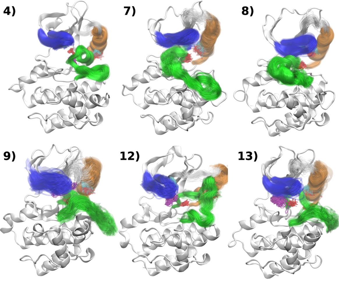
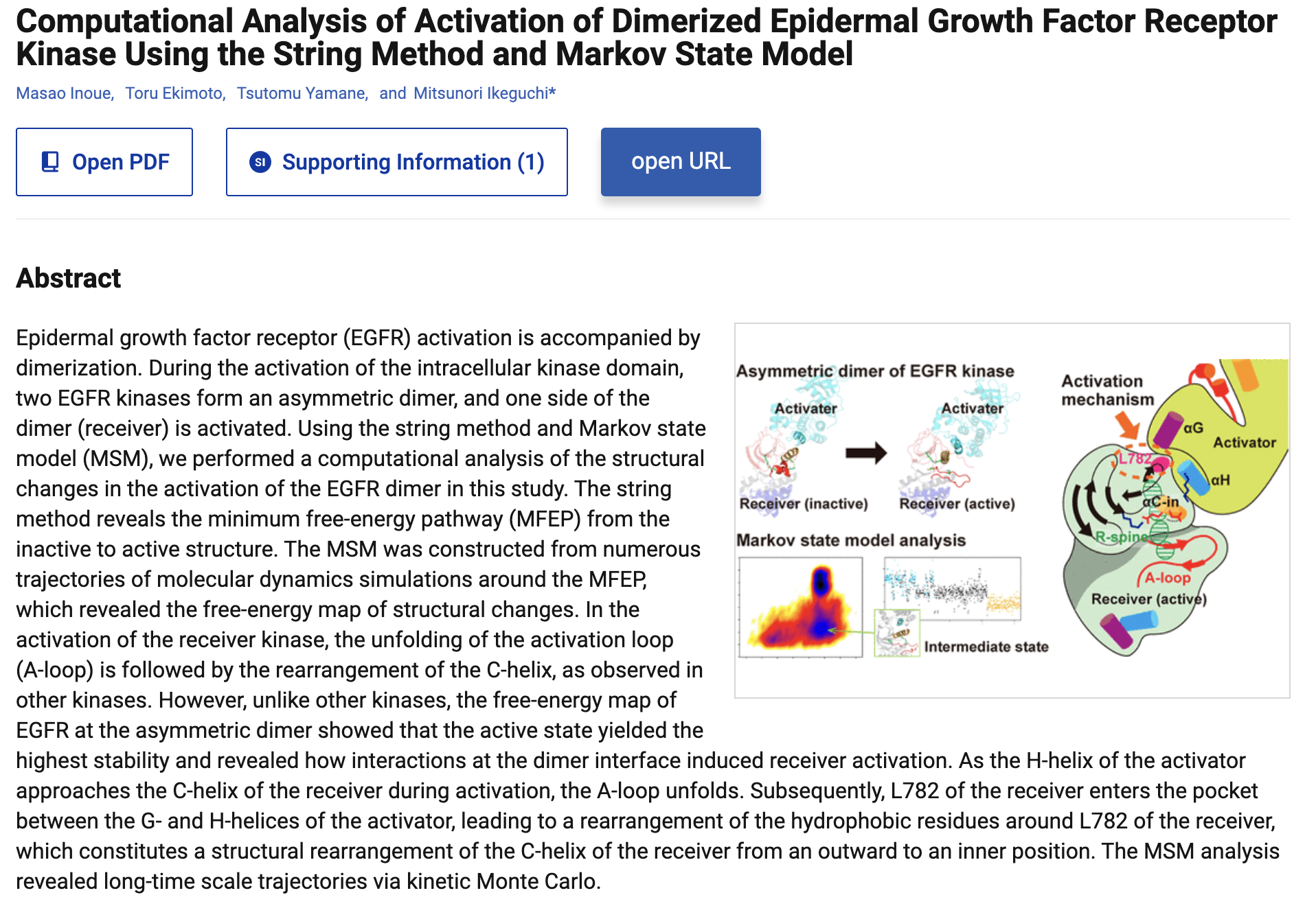
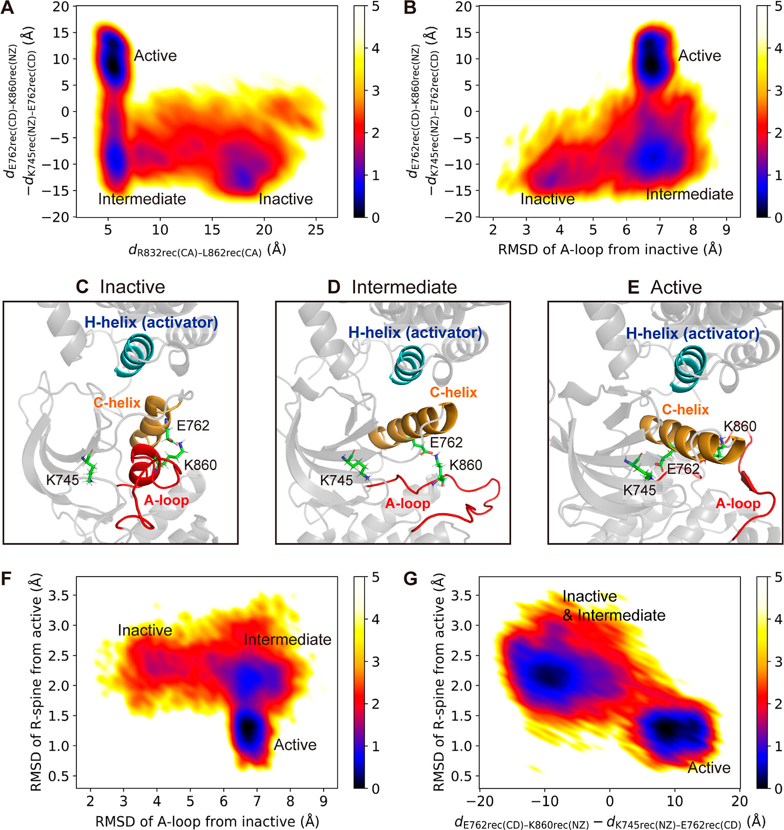
Traditionally, MD studies often involved "look and see" analyses of a few rare events via molecular movies. Although visually appealing, these analyses may be misleading as they do not supply the statistical relevance of such observations in the ensemble, and may miss rare but important events altogether. Another frequent approach is to project the dynamics onto one or two user-defined order parameters with the notion that these order parameters allow the slow kinetics of the molecule to be resolved. ... these projection techniques have been shown to disguise the true and often complex nature of the kinetics..." -- Noe et al.
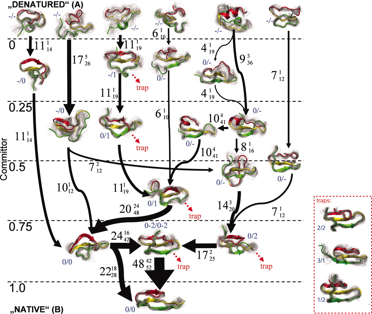
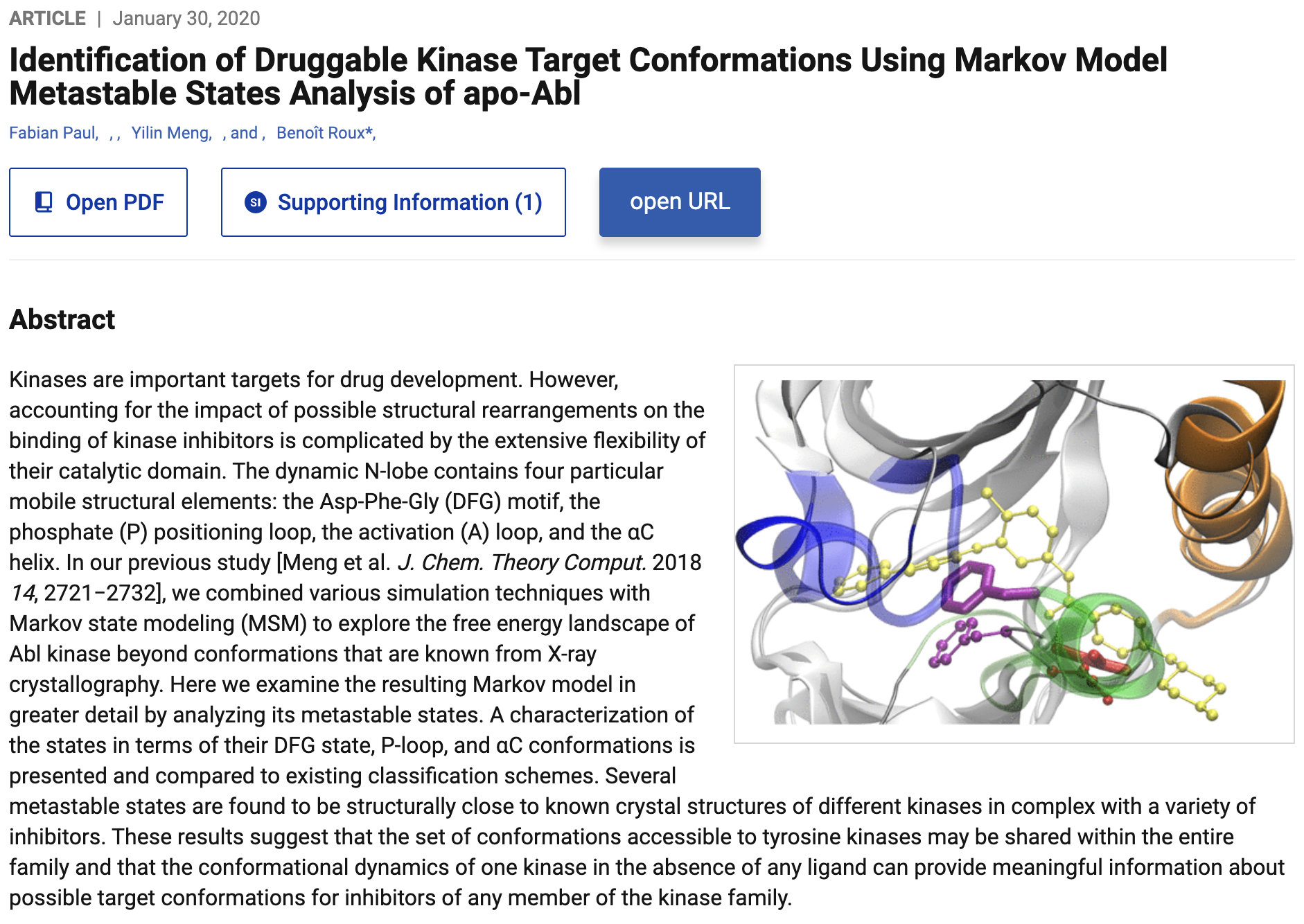
Key Takeaways
Markov State Models (MSMs) describe long-timescale molecular dynamics as transitions between discrete states at a lag time $\tau$.
Good states should capture the slow dynamics: $$\text{features} \rightarrow \text{TICA} \rightarrow \text{clustering} \rightarrow \text{states}$$
The transition matrix encodes the dynamics: $$T_{ij}=P(X_{t+\tau}=j\mid X_t=i)$$
The $\lambda=1$ mode describes the stationary distribution: $$\boldsymbol{\pi}T=\boldsymbol{\pi}$$
Each eigenvalue defines a relaxation timescale: $$t_i=-\frac{\tau}{\ln|\lambda_i|}$$
MSMs combine many short trajectories into a model of equilibrium populations and long-timescale kinetics.