%%html
<script src="https://bits.csb.pitt.edu/preamble.js"></script>
Final thoughts on Markov State Models...

Binding
$$\Delta G^\circ_{\mathrm{bind}} = RT \ln K_d$$
$$\Delta G^\circ_{\mathrm{bind}} = \Delta G_{\mathrm{bind}} + \Delta G_V$$
where $$\Delta G_V = −k_\text{B} T \log\left( \frac{V_\mathrm{sim}}{V_0} \right)$$
where $V_\mathrm{sim}$ is the simulation volume and $V_0$ is the volume needed to achieve 1M concentration and $\Delta G_V$ is a translational entropy (standard-state) correction that accounts for the ligand concentration implied by the simulation box.
$$ \Delta G_{\mathrm{bind}} \approx \Delta F_{\mathrm{bind}} = -k_{\text{B}}T\ln \frac{Z_\mathrm{bound}}{Z_\mathrm{unbound}} = -k_{\text{B}} T \ln \frac{\int_\mathrm{bound} e^{-U(\mathbf{r})/k_\text{B}T}d\mathbf{r}}{\int_\mathrm{unbound} e^{-U(\mathbf{r})/k_\text{B}T}d\mathbf{r}}$$
Most drugs are inhibitors
A competitive inhibitor or orthosteric inhibitor displaces the natural substrate. Imatinib binds to the ATP binding site of Abl tyrosine kinase.
v = py3Dmol.view(width=800,height=450,data=[[imatinib,atp]],viewergrid=(1,2),js='https://3dmol.org/build/3Dmol.js'); v.setStyle({'cartoon':{'color':'lightgray'},'stick':{'radius':.1}}); v.setStyle({'resn':'112'},{'stick':{'colorscheme':'greenCarbon'}}); v.setStyle({'resn':'STI'},{'stick':{'colorscheme':'cyanCarbon'}}); v.zoomTo({'resn':['STI','112']}); v.show();
3Dmol.js failed to load for some reason. Please check your browser console for error messages.
Retrovir/zidovudine/azidothymidine (AZT) is a nucleoside mimic that inhibits HIV reverse transcriptase.
v = py3Dmol.view('1n5y',style='cartoon',width=800); v.setStyle({'resn':'ATM'},'sphere'); v.zoomTo({'resn':'ATM'}); v.show();
3Dmol.js failed to load for some reason. Please check your browser console for error messages.
v = py3Dmol.view('7SIL',style={'cartoon':{'color':'spectrum'}},width=800,height=450); v.setStyle({'resn':'9IG'},'stick'); v.setStyle({'resn':'CA'},{'sphere':{'color':'#00ff00'}}); v.zoomTo({'resn':'9IG'}); v.show();
3Dmol.js failed to load for some reason. Please check your browser console for error messages.
Binding Involves Varying Degrees of Conformational Change
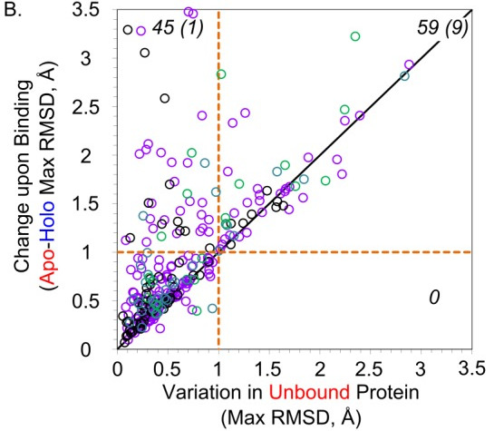
Apo: Unbound structure Holo: Bound structure
The difference in backbone RMSD between apo/holo is more than the variation within holo structures (but quite a few change very little).
Example: Estrogen Receptor Alpha
v = py3Dmol.view(width=800,data=eractive,style='cartoon'); v.setStyle({'cartoon':{'colorscheme':'blueCarbon'},'stick':{'radius':0.1,'colorscheme':'blueCarbon'}}); v.addModel(erinactive); v.setStyle({'model':1},{'cartoon':{'colorscheme':'yellowCarbon'},'stick':{'radius':0.1,'colorscheme':'yellowCarbon'}}); v.setStyle({'resn':'ESE'},{'stick':{'colorscheme':'cyanCarbon'}}); v.setStyle({'resn':'E4D'},{'stick':{'colorscheme':'orangeCarbon'}}); v.zoomTo({'resn':'E4D'}); v.show();
3Dmol.js failed to load for some reason. Please check your browser console for error messages.
%%html
<div id="erantag" style="width: 500px"></div>
<script>
    var divid = '#erantag';
	jQuery(divid).asker({
	    id: divid,
	    question: "Which molecule binds to the blue structure?",
		answers: ["Cyan","Orange"],
        server: "https://bits.csb.pitt.edu/asker.js/example/asker.cgi",
		charter: chartmaker})

$(".jp-InputArea .o:contains(html)").closest('.jp-InputArea').hide();


</script>
Models of binding conformational change
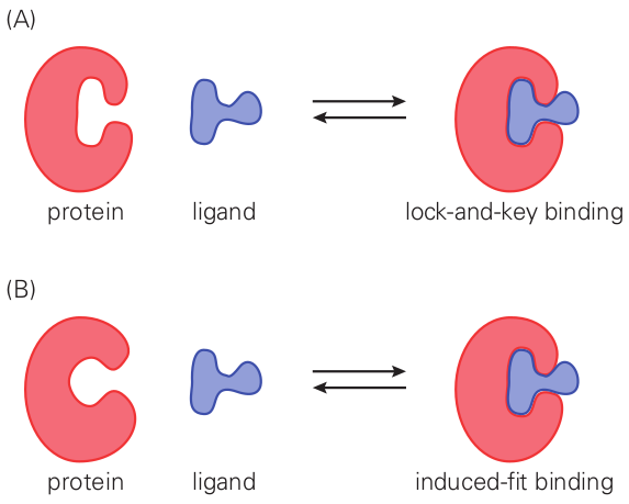
- Lock and key
- Induced fit
- Conformational selection
From: Molecules of Life: Physical and Chemical Principles
Conformational Selection
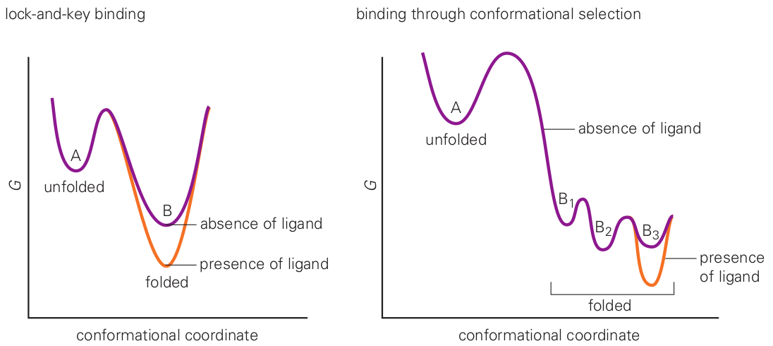
What does induced fit look like?
From: Molecules of Life: Physical and Chemical Principles
Conformational sampling in action
Imatinib prefers to bind the inactive form of ABL kinase which differs from the active form mostly due to the conformation of the activation loop.
v = py3Dmol.view(width=800,data=imat,style={'cartoon': {'colorscheme': 'rasmol'}}); v.setStyle({'resi': '381-409'},{'cartoon':{'color':'red'}}); v.setStyle({'resn':'STI'},'sphere'); v.addModel(dasatinib); v.setStyle({'model':1},{'cartoon': {'colorscheme':'whiteCarbon','opacity':0.75}}); v.setStyle({'model': 1, 'resi': '381-409'},{'cartoon':{'color':'#ff4444','opacity':0.75}}); v.show();
3Dmol.js failed to load for some reason. Please check your browser console for error messages.
%%html
<div id="imatinact" style="width: 500px"></div>
<script>
    var divid = '#imatinact';
	jQuery(divid).asker({
	    id: divid,
	    question: "Which is the inactive conformation?",
		answers: ["Opaque","Transparent"],
        server: "https://bits.csb.pitt.edu/asker.js/example/asker.cgi",
		charter: chartmaker})

$(".jp-InputArea .o:contains(html)").closest('.jp-InputArea').hide();


</script>
Although the active form is similar across kinases, the inactive form is more structurally diverse, e.g. the inactive form of Src (transparent) kinase isn't compatible with imatinib binding. Imatinib's preference for inactive Abl kinase gives it selectivity.
v = py3Dmol.view(width=800,data=imat,style={'cartoon': {'colorscheme': 'rasmol'}}); v.setStyle({'resi': '381-409'},{'cartoon':{'color':'red'}}); v.setStyle({'resn':'STI'},'sphere');v.addModel(inactivesrc);v.setStyle({'model':1},{'cartoon': {'colorscheme':'whiteCarbon','opacity':0.75}});v.setStyle({'model': 1, 'resi': '404-432'},{'cartoon':{'color':'#ff4444','opacity':0.75}}); v.show();
3Dmol.js failed to load for some reason. Please check your browser console for error messages.
Protein conformation changes can result in weaker affinities
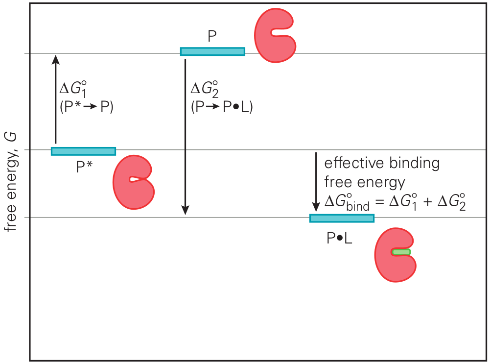
The ligand has to "pay the cost" of the protein re-arrangement.
From: Molecules of Life: Physical and Chemical Principles
Dasatinib binds to the active kinase form and is 350X more potent than imatinib against Abl, but is substantially less kinase-selective than imatinib.
v = py3Dmol.view(width=800,data=imat,style={'cartoon': {'colorscheme': 'rasmol'}}); v.setStyle({'resi': '381-409'},{'cartoon':{'color':'white'}}); v.setStyle({'resn':'STI'},{'stick':{'colorscheme':'Jmol'}}); v.addModel(dasatinib); v.setStyle({'model':1},{'cartoon': {'color':'lightgreen'}}); v.setStyle({'resn':'1N1'},{'stick':{'colorscheme':'greenCarbon'}}); v.setStyle({'model': 1, 'resi': '381-409'},{'cartoon':{'color':'#ddffdd'}}); v.show();
3Dmol.js failed to load for some reason. Please check your browser console for error messages.
Components of binding
$$\Delta G_\mathrm{bind}^\circ = \Delta H - T \Delta S$$
$\Delta H$ is the enthalpy, which if $p\Delta V$ is small and temperature is constant, is well approximated as the change in average potential energy:

http://hyperphysics.phy-astr.gsu.edu/hbase/thermo/helmholtz.html
Components of binding
Conceptually, we can assign changes to the protein/ligand/solvent and their interactions (in reality these contributions are coupled and not uniquely separable).
$$\Delta G_\mathrm{bind}^\circ = \Delta H_{RL} + \Delta H_{RS} + \Delta H_{LS} + \Delta H_{R} + \Delta H_{L}+ \Delta H_{S} - T (\Delta S_{R} + \Delta S_{L} + \Delta S_{S})$$
Which terms do you think will (typically) matter the most?
Will binding ever be entropy driven (loss of translational+rotational entropy is $\approx$ 10-15 kcal/mol).
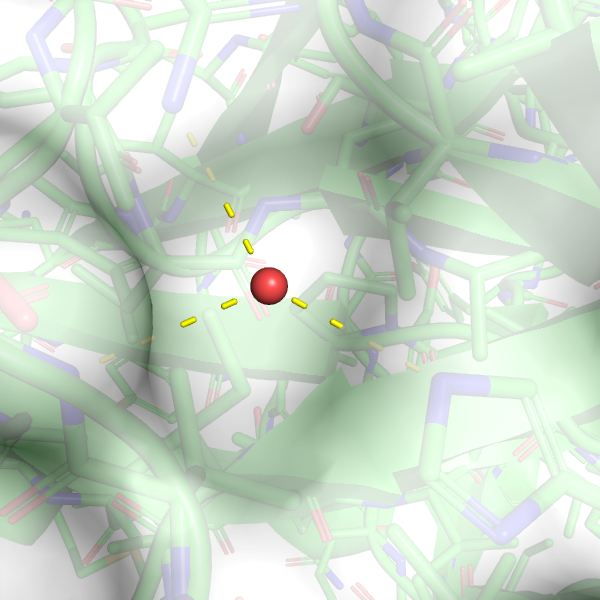
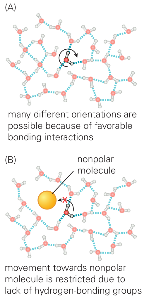
Potency is often driven by returning binding-site waters to bulk
From: Molecules of Life: Physical and Chemical Principles
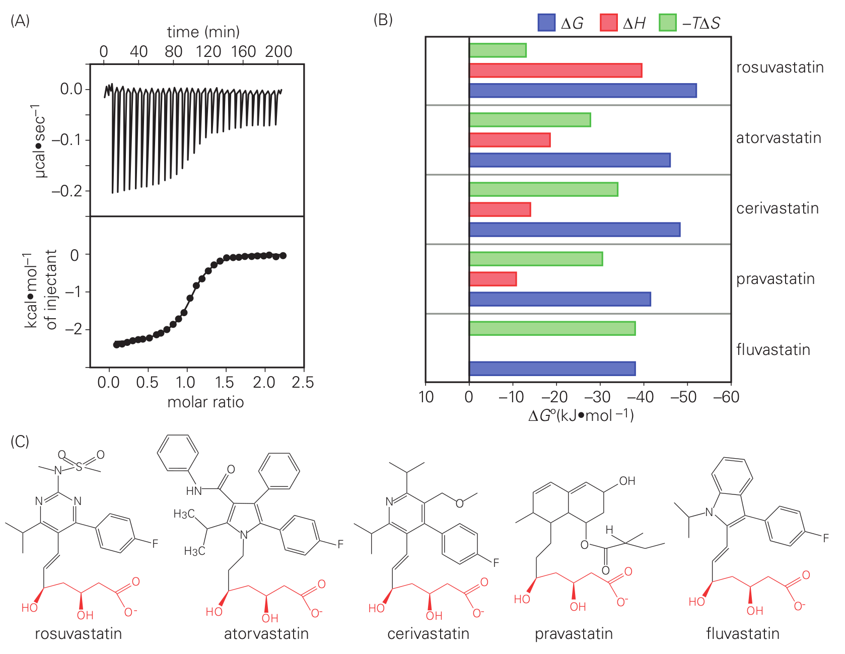
Entropy-Enthalpy Compensation
From: Molecules of Life: Physical and Chemical Principles
%%html
Rosuvastatin
v = py3Dmol.view('1hwl',width=800); v.setStyle({'cartoon':{'colorscheme':'whiteCarbon'},'stick':{'radius':0.1, 'colorscheme':'whiteCarbon'}}); v.setStyle({'resn':'FBI'},{'stick':{'colorscheme':'greenCarbon'}}); v.zoomTo({'chain':'A','resn':'FBI'});v.addSurface('VDW',{'colorscheme':'whiteCarbon','opacity':.9},{'hetflag':False}); v.show();
3Dmol.js failed to load for some reason. Please check your browser console for error messages.
Cerivastatin
v = py3Dmol.view('1hwj',width=800); v.setStyle({'cartoon':{'colorscheme':'whiteCarbon'},'stick':{'radius':0.1, 'colorscheme':'whiteCarbon'}}); v.setStyle({'resn':'116'},{'stick':{'colorscheme':'cyanCarbon'}}); v.zoomTo({'chain':'A','resn':'116'});v.addSurface('VDW',{'colorscheme':'whiteCarbon','opacity':.9},{'hetflag':False}); v.show();
3Dmol.js failed to load for some reason. Please check your browser console for error messages.
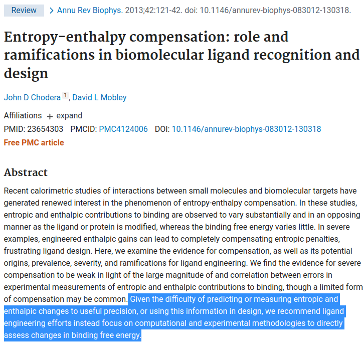
Thermodynamic (Free Energy) Cycles
Free energy is a state function. It does not depend on how you arrived at the state.
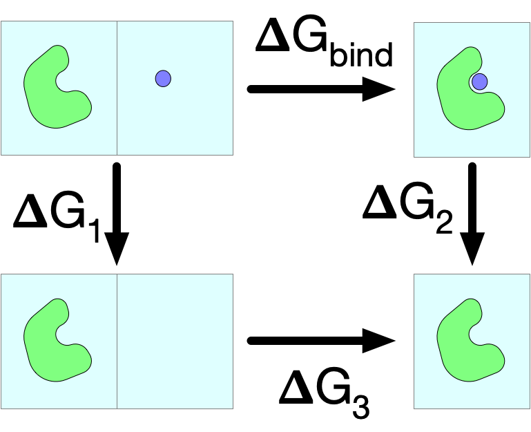
Relative Free Energy Cycle
%%html
<div id="absrelacc" style="width: 500px"></div>
<script>
    var divid = '#absrelacc';
	jQuery(divid).asker({
	    id: divid,
	    question: "Which do you think would be more accurate?",
		answers: ["ΔG","ΔΔG"],
        extra: ["Absolute free energy prediction","Relative free energy prediction"],
        server: "https://bits.csb.pitt.edu/asker.js/example/asker.cgi",
		charter: chartmaker})

$(".jp-InputArea .o:contains(html)").closest('.jp-InputArea').hide();


</script>
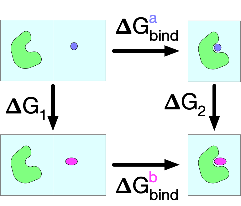
Absolute Cycle
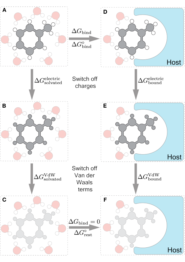
Annihilation is when we completely remove a molecule from the system.
Decoupling is when we remove interactions between molecules from the system. Typically we will decouple the ligand from the receptor and solvent (but keep intramolecular interactions).
Reminder: Amber forcefield: $$\tiny U(r^N)=\sum_\text{bonds} k_b (l-l_0)^2 + \sum_\text{angles} k_a (\theta - \theta_0)^2 + \sum_\text{torsions} \frac{1}{2} V_n [1+\cos(n \omega- \gamma)] $$ $$\tiny +\sum_{j=1} ^{N-1} \sum_{i=j+1} ^N \biggl\{\epsilon_{i,j}\biggl[\left(\frac{r_{0ij}}{r_{ij}} \right)^{12} - 2\left(\frac{r_{0ij}}{r_{ij}} \right)^{6} \biggr]+ \frac{q_iq_j}{4\pi \epsilon_0 r_{ij}}\biggr\} $$
Why decouple in two steps?
How to mutate
Define a coupling parameter $\lambda$ of the potential energy function $U$ that controls the contribution of the change:
$$ U(r^N,\lambda)= \sum_{j \in \text{not ligand}} \sum_{i \in \text{ligand}} \mathbf{\lambda} \epsilon_{i,j}\biggl[\left(\frac{r_{0ij}}{r_{ij}} \right)^{12} - 2\left(\frac{r_{0ij}}{r_{ij}} \right)^{6} \biggr] + \sum_\text{all other}\sum_\text{pairs} \epsilon_{i,j}\biggl[\left(\frac{r_{0ij}}{r_{ij}} \right)^{12} - 2\left(\frac{r_{0ij}}{r_{ij}} \right)^{6} \biggr] + \cdots$$
For notational convenience, we define the reduced potential energy $$u(r^N,\lambda) = \frac{U(r^N,\lambda)}{k_\text{B}T}$$
And similarly, a reduced free energy $f$. This is only to avoid writing $k_\text{B}T$ a lot. The change in free energy between two order parameters is:
$$\Delta f = - \ln \frac{Z(\lambda_B)}{Z(\lambda_A)} = - \ln \frac{\int e^{-u(r^N, \lambda_B)}}{\int e^{-u(r^N, \lambda_A)}}$$
Free energy perturbation
You can calculate the free energy change of this perturbation ($\lambda_A \rightarrow \lambda_B$) using the Zwanzig equation:
$$ \Delta f = - \ln \frac{\int e^{-u(\mathbf{r}^N,\lambda_B)}\,d\mathbf{r}^N} {\int e^{-u(\mathbf{r}^N,\lambda_A)}\,d\mathbf{r}^N} = - \ln \frac{\int e^{-u(\mathbf{r}^N,\lambda_B)+u(\mathbf{r}^N,\lambda_A)-u(\mathbf{r}^N,\lambda_A)}\,d\mathbf{r}^N} {\int e^{-u(\mathbf{r}^N,\lambda_A)}\,d\mathbf{r}^N} = \\ - \ln \frac{\int e^{-\Delta u_{B-A}(\mathbf{r}^N)}e^{-u(\mathbf{r}^N,\lambda_A)}\,d\mathbf{r}^N} {\int e^{-u(\mathbf{r}^N,\lambda_A)}\,d\mathbf{r}^N} $$
What happens when all the conformations sampled in the $\lambda_A$ MD are high energy states with respect to $u(\mathbf{r}^N, \lambda_B)$?
Zwanzig Example
Zwanzig relation with two 1D Gaussian (harmonic) states ($k_BT$ = 1).
%%capture
sigma_A = 1.0
sigma_B = 2.0

def U_gauss(x, sigma):
    # Harmonic potential with variance sigma^2; up to a constant, U(x)=x^2/(2 sigma^2)
    return (x**2) / (2.0 * sigma**2)

xplot = np.linspace(-8.0, 8.0, 2001)
pdf_A = (1.0/(sigma_A*sqrt(2*pi))) * np.exp(-xplot**2/(2*sigma_A**2))
pdf_B = (1.0/(sigma_B*sqrt(2*pi))) * np.exp(-xplot**2/(2*sigma_B**2))
fig1 = plt.figure(figsize=(6,4)); plt.plot(xplot, pdf_A, label=r"PDF A (σ=1); $U = \frac{x^2}{2}$");plt.plot(xplot, pdf_B, label=r"PDF B (σ=2); $U = \frac{x^2}{8}$");plt.xlabel("x");plt.ylabel("Probability density");plt.title("Two Gaussian states (Z_B/Z_A = 2)");plt.legend();plt.tight_layout();
fig1

def Z_numeric(sigma, L=20.0, n=400_001):
    # Numerically integrate Z = ∫ exp(-U(x)) dx over [-L, L]
    # For Gaussians, taking L=20 is extremely safe.
    x = np.linspace(-L, L, n, dtype=np.float64)
    U = U_gauss(x, sigma)
    integrand = np.exp(-U)
    Z = np.trapezoid(integrand, x)
    return Z

# 1) Numerical partition functions and ratio
Z_A_num = Z_numeric(sigma_A, L=20.0, n=400_001)
Z_B_num = Z_numeric(sigma_B, L=20.0, n=400_001)

ratio_num = Z_B_num / Z_A_num
ratio_exact = sigma_B / sigma_A  # since Z = sigma * sqrt(2*pi) when kT=1

F_A_num = -np.log(Z_A_num)
F_B_num = -np.log(Z_B_num)
DeltaF_exact = -np.log(ratio_exact)  # F_B - F_A
print("=== Partition functions ===")
print(f"Z_A (numeric): {Z_A_num:.8f}")
print(f"Z_B (numeric): {Z_B_num:.8f}")
print(f"Z_B/Z_A (numeric): {ratio_num:.8f}")
print(f"Z_B/Z_A (exact):   {ratio_exact:.8f}")
print()
print("=== Free energies ===")
print(f"F_A (numeric): {F_A_num:.8f}")
print(f"F_B (numeric): {F_B_num:.8f}")
print(f"ΔF = F_B - F_A (exact): {-np.log(2):.8f}")
=== Partition functions ===
Z_A (numeric): 2.50662827
Z_B (numeric): 5.01325655
Z_B/Z_A (numeric): 2.00000000
Z_B/Z_A (exact):   2.00000000

=== Free energies ===
F_A (numeric): -0.91893853
F_B (numeric): -1.61208571
ΔF = F_B - F_A (exact): -0.69314718
A_samples = rng.normal(loc=0.0, scale=sigma_A, size=10000)
fig1 = plt.figure(figsize=(6,4)); plt.plot(xplot, pdf_A, label=r"PDF A (σ=1); $U = \frac{x^2}{2}$");plt.plot(xplot, pdf_B, label=r"PDF B (σ=2); $U = \frac{x^2}{8}$");plt.xlabel("x");plt.ylabel("Probability density");plt.title("Two Gaussian states (Z_B/Z_A = 2)");plt.hist(A_samples,density=True,bins=100,label='A samples');plt.legend();plt.tight_layout();plt.show();

$$\Large -\ln \left\langle e^{-\Delta u_{B-A}(\mathbf{r}^N)} \right\rangle_{\mathbf{A}} \approx -\ln \left[ \frac{1}{N} \sum_{n=1}^{N} e^{-\Delta u_{B-A}(\mathbf{r}_n^N)} \right] $$
UA = U_gauss(A_samples,sigma_A)
UB = U_gauss(A_samples,sigma_B)
-np.log(np.mean(np.exp(-(UB-UA))))
-0.7165509023724014
# 2) Zwanzig relation estimates
def zwanzig_deltaF(samples_x, UA, UB):
    # ΔF = -ln ⟨exp(-(UB-UA)/kT)⟩_A  (kT=1 here)
    dU = UB - UA
    return -np.log(np.mean(np.exp(-dU)))

# Draw samples from each distribution
def sample_from_state(sigma, n):
    return rng.normal(loc=0.0, scale=sigma, size=n)

def free_energy_convergence(n_max=200000, checkpoints=40):
    # return arrays of n and ΔF estimates for both directions
    ns = np.unique(np.round(np.geomspace(200, n_max, checkpoints)).astype(int))
    xs_A_full = sample_from_state(sigma_A, ns[-1])
    xs_B_full = sample_from_state(sigma_B, ns[-1])

    # precompute potentials
    UA_full = U_gauss(xs_A_full, sigma_A)
    UB_on_A_full = U_gauss(xs_A_full, sigma_B)

    UB_full = U_gauss(xs_B_full, sigma_B)
    UA_on_B_full = U_gauss(xs_B_full, sigma_A)

    df_AtoB = []
    df_BtoA = []
    for n in ns:
        df_AtoB.append(zwanzig_deltaF(xs_A_full[:n], UA_full[:n], UB_on_A_full[:n]))
        # Reverse direction gives F_A - F_B; negate to compare with ΔF (B - A)
        df_BtoA.append(-zwanzig_deltaF(xs_B_full[:n], UB_full[:n], UA_on_B_full[:n]))
    return ns, np.array(df_AtoB), np.array(df_BtoA)
ns, df_AtoB, df_BtoA = free_energy_convergence(n_max=200_000, checkpoints=50)
fig2 = plt.figure(figsize=(6,4));plt.plot(ns, df_AtoB, label="ΔF via A→B");plt.plot(ns, df_BtoA, label="ΔF via B→A");plt.axhline(DeltaF_exact, linestyle="--", color='black',label="Exact ΔF = -ln 2");plt.xscale("log");plt.xlabel("Number of samples");plt.ylabel("ΔF estimate (kT units)");plt.title("Zwanzig free energy estimates vs. sample size");plt.legend();plt.tight_layout();plt.show()

print(f"ΔF via Zwanzig A→B at max n: {df_AtoB[-1]:.8f}"); print(f"ΔF via Zwanzig B→A at max n: {df_BtoA[-1]:.8f}")

ΔF via Zwanzig A→B at max n: -0.76180152
ΔF via Zwanzig B→A at max n: -0.69412834
Theory Meets Practice
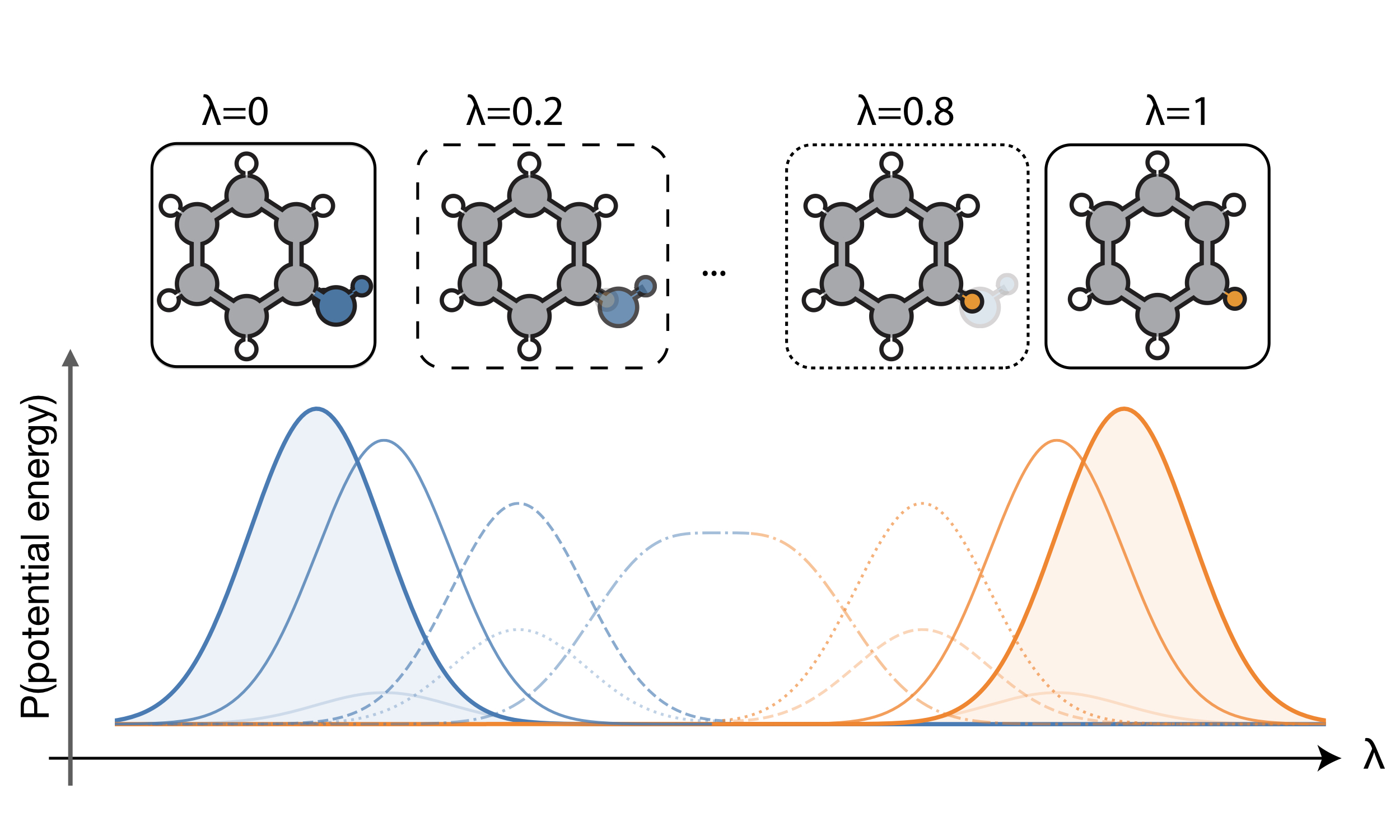
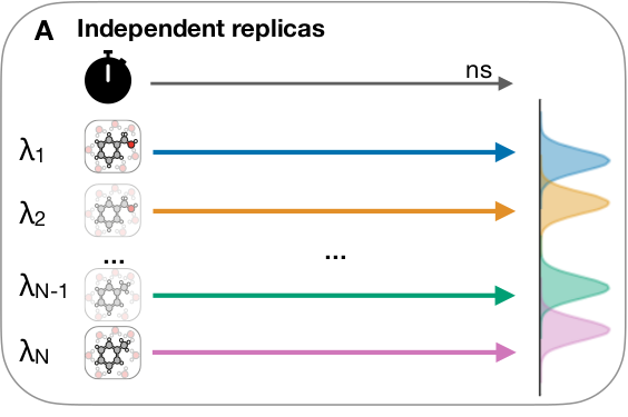
A simulation will mostly sample highly probable states. So there needs to be sufficient overlap in configuration space (the sampled conformations) between $\lambda_A$ and $\lambda_B$.
It is unlikely we will achieve this with a single $\lambda$ step, so instead define a series of alchemical intermediate states $\lambda_0, \lambda_1, \dots \lambda_N$.
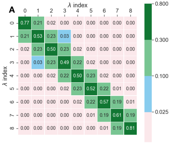
Overlap Checking
Overlap matrices compute the average probability that a sample generated at state $\lambda_j$ can be observed at state $\lambda_i$.
Vocabulary
- orthosteric - primary binding site
- allosteric - modulation of protein by binding away from primary site
- apo - unbound structure
- holo - bound structure
Key Concepts
- Contributions to binding
- Models of binding
- Lock and key
- Conformational selection
- Induced fit
- Thermodynamic (free energy) cycles
- Alchemical transformations