%%html
<script src="https://bits.csb.pitt.edu/preamble.js"></script>
<style>:root {--jp-cell-prompt-width: 32px}</style>
Alchemical Free Energy Computation
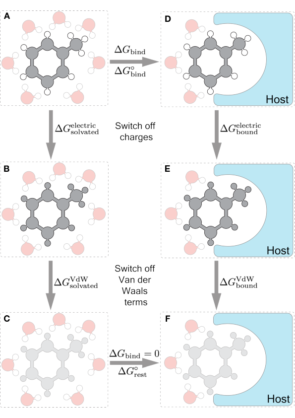
Define a coupling parameter $\lambda$ of the potential energy function $U$ that controls the contribution of the change:
$$ U(r^N,\lambda)= \sum_{j \in \text{not ligand}} \sum_{i \in \text{ligand}} \mathbf{\lambda} \epsilon_{i,j}\biggl[\left(\frac{r_{0ij}}{r_{ij}} \right)^{12} - 2\left(\frac{r_{0ij}}{r_{ij}} \right)^{6} \biggr] + \sum_\text{all other}\sum_\text{pairs} \epsilon_{i,j}\biggl[\left(\frac{r_{0ij}}{r_{ij}} \right)^{12} - 2\left(\frac{r_{0ij}}{r_{ij}} \right)^{6} \biggr] + \cdots$$
Free energy perturbation
You can calculate the free energy change of a perturbation ($\lambda_A \rightarrow \lambda_B$) using the Zwanzig equation:
$$ \small \Delta f = - \ln \frac{\int e^{-u(\mathbf{r}^N,\lambda_B)}\,d\mathbf{r}^N} {\int e^{-u(\mathbf{r}^N,\lambda_A)}\,d\mathbf{r}^N} = - \ln \frac{\int e^{-\Delta u_{B-A}(\mathbf{r}^N)}e^{-u(\mathbf{r}^N,\lambda_A)}\,d\mathbf{r}^N} {\int e^{-u(\mathbf{r}^N,\lambda_A)}\,d\mathbf{r}^N} $$
$$\Large \Delta f = -\ln \left\langle e^{-\Delta u_{B-A}(\mathbf{r}^N)} \right\rangle_{\mathbf{A}} \approx -\ln \left[ \frac{1}{N} \sum_{\mathbf{r}_n^N \in \mathrm{MD}_{\lambda_A}} e^{-\Delta u_{B-A}(\mathbf{r}_n^N)} \right] $$ Reminder: $u(r^N)$ is the reduced potential energy $u=U/(k_B T)$ and $f$ is the reduced free energy $f=F/(k_B T)$.
What are we doing again?
We have different potential energy functions...
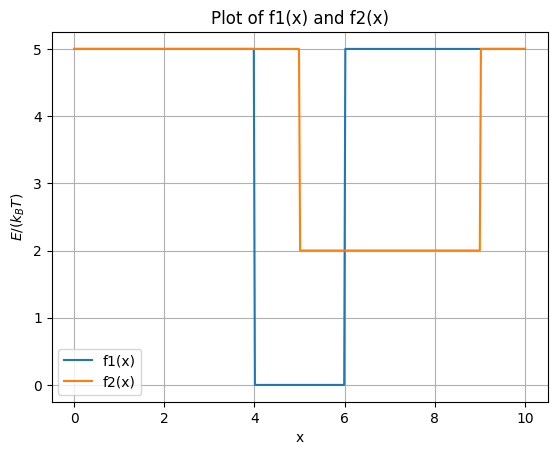
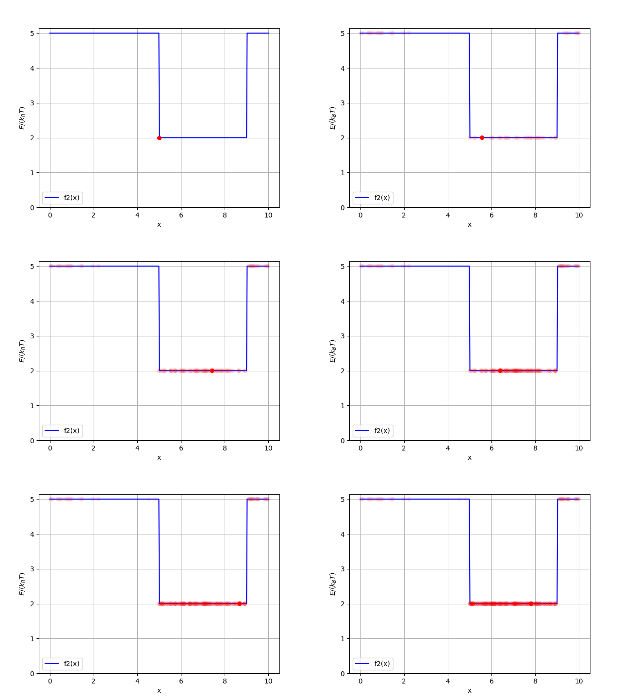
...and we can draw samples (through simulation) from their equilibrium distribution (presumably).
Theory Meets Practice
- How to compute free energy differences between alchemical states?
- How to define alchemical states?
- How to sample alchemical states?
- A statistical issue...
- Evaluation of results?
How to compute free energy differences between alchemical states?
Zwanzig (also called one-sided exponential re-weighting) tends to do the worst - high variance and error when overlap is poor.
- But is one-sided - only need one simulation
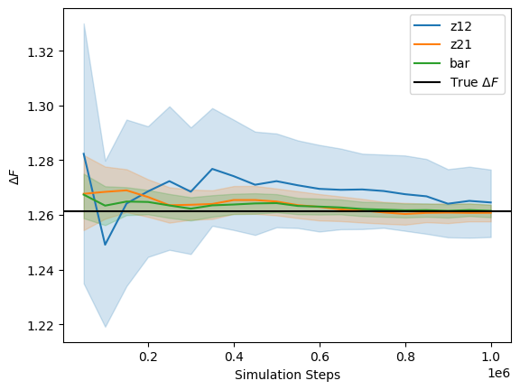
Bennett Acceptance Ratio (BAR)
Estimate the free energy difference using equilibrium samples from both states.
Define $\Delta u_{i,j}(\mathbf{r}^N)=u_j(\mathbf{r}^N)-u_i(\mathbf{r}^N)$ and $\Delta f_{i,j}=f_j-f_i$.
For equal numbers of samples from states $i$ and $j$, solve numerically for $\Delta f_{i,j}$:
$$\Large \begin{eqnarray} \sum_{r^N \in \lambda_i \mathrm{MD}} \frac{1}{1 + e^{\Delta u_{i,j}(r^N) - \Delta f_{i,j}}} \nonumber =\sum_{r^N \in \lambda_{j} \mathrm{MD}} \frac{1}{1 + e^{- \Delta u_{i,j}(r^N) + \Delta f_{i,j}}} \end{eqnarray}$$
- Evaluate both potentials on every sampled configuration.
- Combines information from both directions, emphasizing configurations in the overlap region.
- A maximum-likelihood estimator with asymptotically minimum variance under standard sampling assumptions.
- Usually more statistically efficient than one-sided Zwanzig—but cannot compensate for missing overlap or inadequate sampling.
Shirts MR, Bair E, Hooker G, Pande VS. Equilibrium free energies from nonequilibrium measurements using maximum-likelihood methods. Physical review letters. 2003 Oct 2;91(14):140601. Bennett CH. Efficient estimation of free energy differences from Monte Carlo data. Journal of Computational Physics. 1976 Oct 1;22(2):245-68.
BAR Intuition
$$ \begin{eqnarray} \sum_{r^N \in \lambda_i \mathrm{MD}} \frac{1}{1 + e^{\Delta u_{i,j}(r^N) - \Delta f_{i,j}}} \nonumber =\sum_{r^N \in \lambda_{j} \mathrm{MD}} \frac{1}{1 + e^{- \Delta u_{i,j}(r^N) + \Delta f_{i,j}}} \end{eqnarray}$$
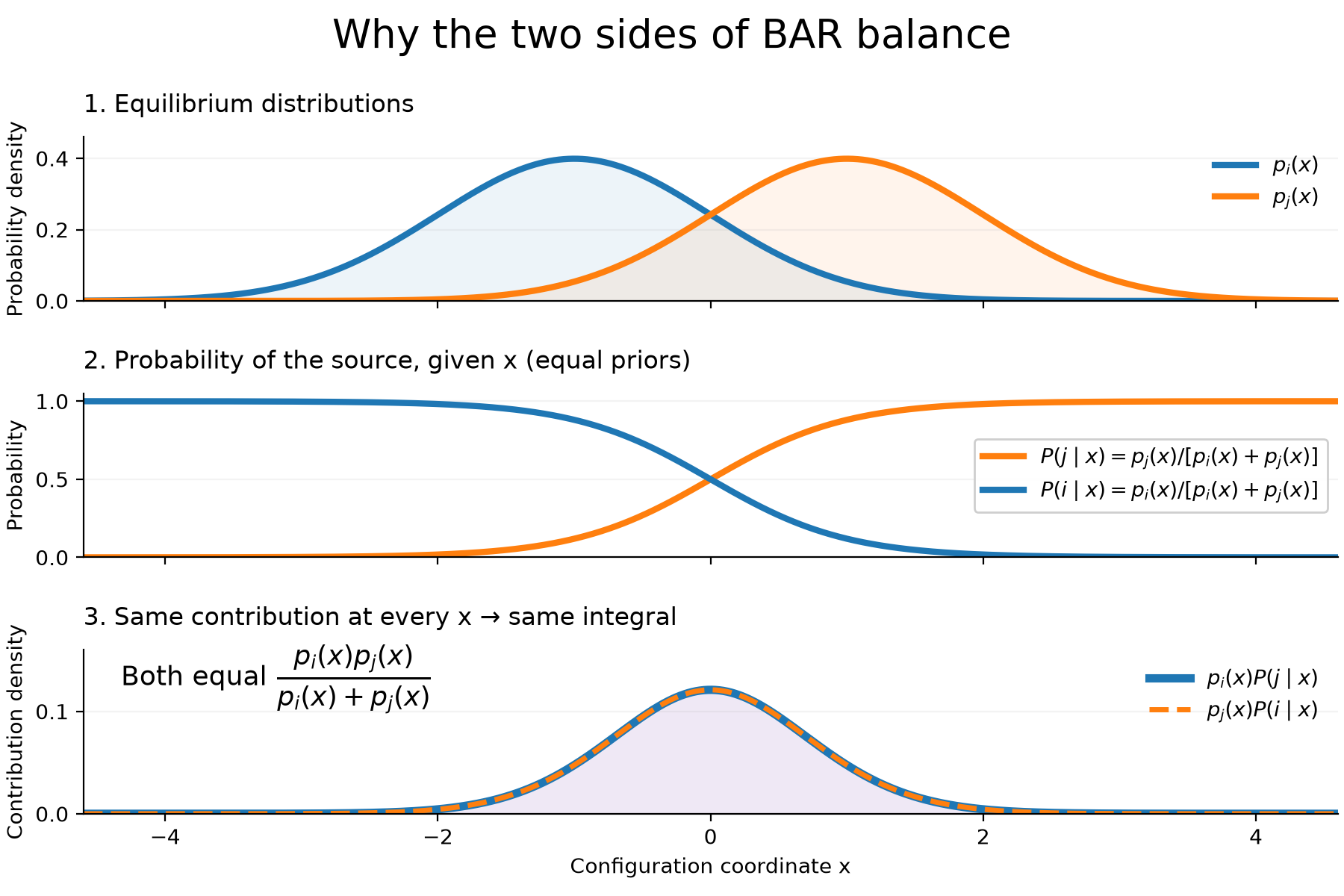
Given a configuration, which simulation probably produced it?
The equilibrium probability density of configuration $\mathbf{r}^N$ in state $j$ is $$ p_j(\mathbf{r}^N)=\frac{e^{-u_j(\mathbf{r}^N)}}{Z_j}. $$ $$ \frac{p_i(r^N)}{p_j(r^N)} = \frac{e^{-u_i(r^N)}/Z_i}{e^{-u_j(r^N)}/Z_j} = e^{\Delta u_{i,j}(r^N) - \Delta f_{i,j}}$$
Pool equal numbers of samples from states $i$ and $j$. By Bayes' rule, the probability that a configuration came from $j$ is $$ P(j\mid\mathbf{r}^N) =\frac{p_j(\mathbf{r}^N)}{p_j(\mathbf{r}^N)+p_i(\mathbf{r}^N)} =\frac{1}{1+e^{\Delta u_{i,j}(\mathbf{r}^N)-\Delta f_{i,j}}}, $$ BAR adjusts $\Delta f$ until the total probability assigned to the opposite source is equal in both sample sets.
Multistate Bennett Acceptance Ratio (MBAR)
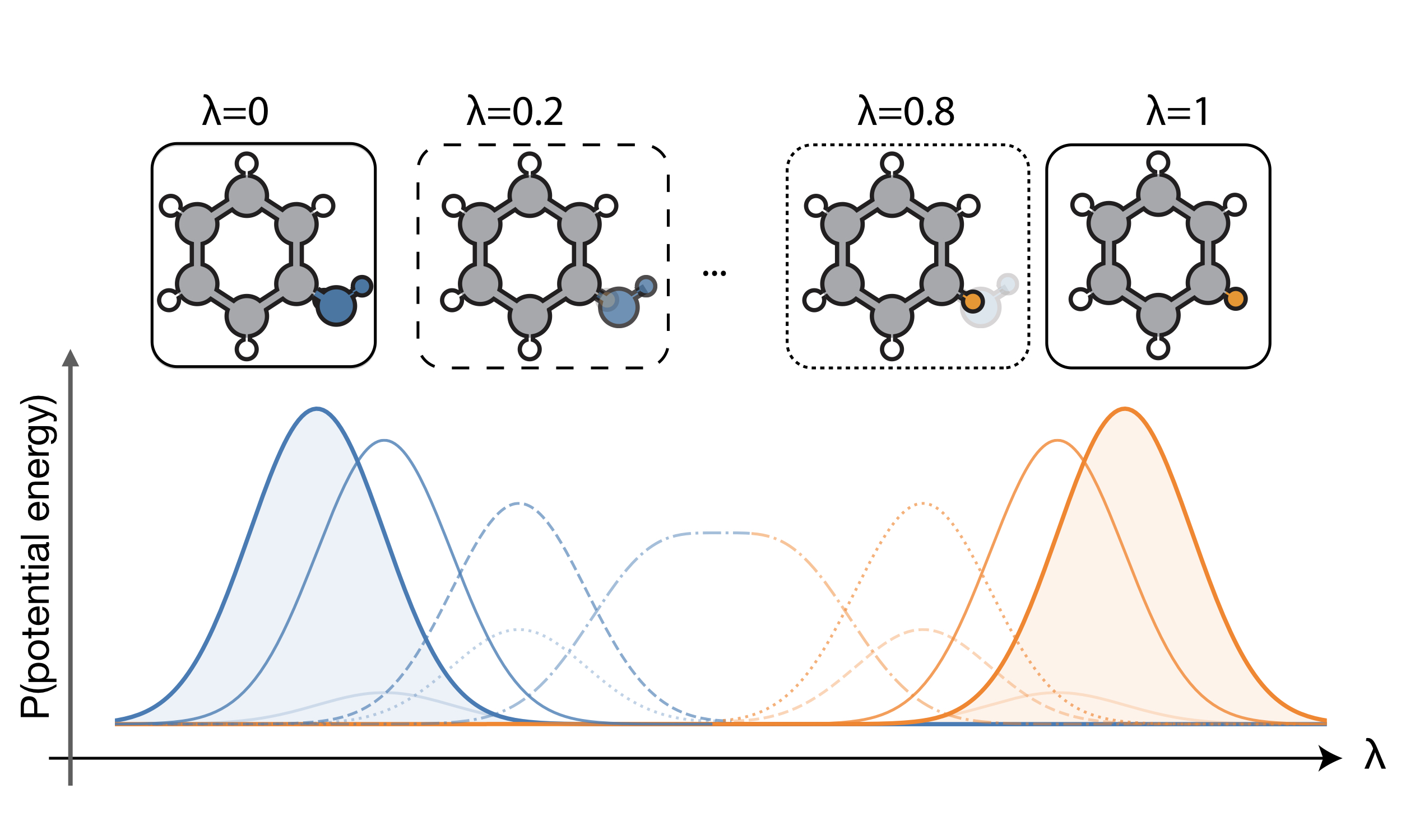
This extends BAR to all states at once. Given $K$ $\lambda_k$ simulations:
$$ f_i = -\ln \sum_{n=1}^{N_{\mathrm{tot}}} \frac{e^{-u_i(\mathbf{r}_n^N)}} {\sum_{k=1}^{K} N_k e^{f_k-u_k(\mathbf{r}_n^N)}}. $$
We solve (numerically) for the $K$ free energies $f_k$. There are nice packages to do this (pymbar).
When will MBAR be overkill?
Thermodynamic Integration
With TI we use the derivatives of the free energy with respect to $\lambda$. This is less sensitive to overlap requirements, but suffers from bias in the numerical quadrature (integration).
$$ \frac{df}{d\lambda} = \frac{d}{d\lambda}\left[-\ln Z(\lambda)\right] = \frac{d}{d\lambda}\left[ -\ln \int e^{-u(\mathbf{r}^N,\lambda)}\,d\mathbf{r}^N \right] = \left\langle \frac{\partial u(\mathbf{r}^N,\lambda)}{\partial\lambda} \right\rangle_\lambda $$
$$ \Delta f = \int_0^1 \left\langle \frac{\partial u(\mathbf{r}^N,\lambda)}{\partial\lambda} \right\rangle_\lambda\,d\lambda \approx \sum_{k=1}^{K} w_k \left\langle \frac{\partial u(\mathbf{r}^N,\lambda)}{\partial\lambda} \right\rangle_{\lambda_k} $$
where the weights $w_k$ correspond to a particular choice of numerical integration.
This requires that we compute $\frac{\partial}{\partial\lambda}u(\mathbf{r}^N,\lambda)$
When is that easy?
$$U_\lambda(\mathbf r)=\lambda U(\mathbf r) \quad\Longrightarrow\quad \frac{dF}{d\lambda} =\left\langle\frac{\partial U_\lambda}{\partial\lambda}\right\rangle_\lambda =\boxed{\langle U(\mathbf r)\rangle_\lambda}$$
Defining the Alchemical State
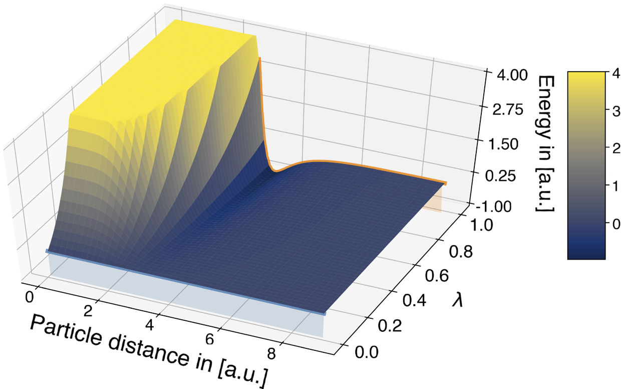
Especially with TI, a simple linear scaling, $U(r_N, \lambda) = \lambda U(r_N)$, has numerical issues. (Why?)
Instead, a soft-core potential is used:
$$U({r_N},\lambda) = 4\epsilon_{ij} {\lambda} \left(\frac{1}{(\alpha(1-{\lambda}) + (r_{ij}/\sigma_{ij})^6)^2} - \frac{1}{\alpha(1-{\lambda}) + (r_{ij}/\sigma_{ij})^6}\right)$$
How to sample alchemical states?
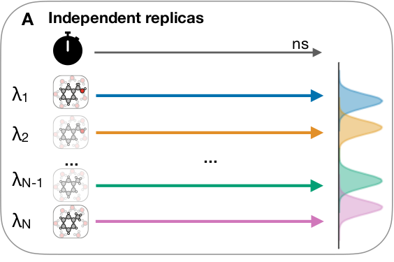
Simplest method is independent trajectories (replicas).
What are the distributions on the right?
Metropolis-Hastings
The Metropolis–Hastings algorithm can draw samples from any probability distribution with probability density $P(x)$, provided that we know a function $f(x)$ proportional to the density $P$ and the values of $f(x)$ can be calculated Wikipedia.
Initialization:
- Need $g(x\mid y)$ that suggests a candidate for the next sample value $x$, given the previous sample value $y$. This is defined using a move set of perturbations you can apply to your system and might be called the proposal density or jumping distribution. Typically $g(x\mid y) = g(y\mid x)$, if not Hastings provides a correction.
- Need $f(x)$ whose value is proportional to $P(x)$
- Pick an initial configuration $x_0$
Metropolis-Hastings (continued)
For each iteration $t$:
- Generate a candidate $x'$ for the next sample by picking from the distribution $g(x'\mid x_t)$
- Calculate the acceptance ratio $\alpha = f(x')/f(x_t)$ (for symmetric proposals $g(x'\mid x)=g(x\mid x')$)
- $\alpha = f(x')/f(x_t) = P(x')/P(x_t)$
- Accept or reject:
- Generate a uniform random number $r_u \in [0, 1]$
- If $r_u \le \alpha$, then accept: $x_{t+1} = x'$
- If $r_u > \alpha$, then reject: $x_{t+1} = x_t$
Why does this work?
We are essentially constructing (a very very large) Markov state model with transition probabilities $P(x'\mid x)$
If the transition probabilities fulfills detailed balance: $$P(x'\mid x)P(x) = P(x\mid x')P(x')$$
then there exists a stationary distribution $\pi$. That is, under reasonable assumptions (e.g. ergodicity), enough sampling will converge to $P(x)$.
With Metropolis, the transition probability is the product of the acceptance probability $A$ and the proposal probability $g$:
$$P(x'|x) = g(x'|x) A(x',x)$$
Plug this into the detailed balance equation and show that $$A(x', x) = \min\left(1, \frac{P(x')}{P(x)} \frac{g(x \mid x')}{g(x' \mid x)}\right)$$ fullfills detailed balance.
MCMC: Markov chain Monte Carlo
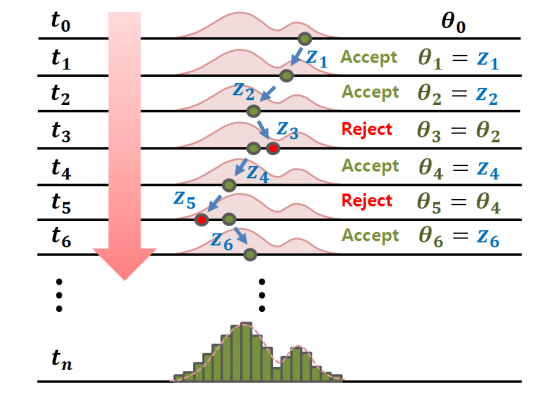
Metropolis-Hastings is one of a family of algorithms for stochastically sampling a probability distribution by constructing a Markov chain.
Although the algorithm produces a trajectory of states, it does not produce correct dynamics. What does this mean?
Ideally MCMC will get to equilibrium faster than traditional dynamics.
Move set can be non-physical, but must be ergodic.
Assign2/3 Revisited
import openmm
from openmm.app import *
from openmm import *
from openmm.unit import *
import numpy as np
import matplotlib
import matplotlib.pyplot as plt
import scipy, os
import argparse
import scipy.signal

def dihedral(p1, p2, p3, p4):
    '''Return dihedral angle in radians between provided points.
    This is the same calculation used by OpenMM for force calculations. '''
    v12 = np.array(p1-p2)
    v32 = np.array(p3-p2)
    v34 = np.array(p3-p4)

    #compute cross products
    cp0 = np.cross(v12,v32)
    cp1 = np.cross(v32,v34)

    #get angle between cross products
    dot = np.dot(cp0,cp1)
    if dot != 0:
        norm1 = np.dot(cp0,cp0)
        norm2 = np.dot(cp1,cp1)
        dot /= np.sqrt(norm1*norm2)

    if dot > 1.0:
        dot = 1.0
    elif dot < -1.0:
        dot = -1.0

    if dot > 0.99 or dot < -0.99:
        #close to acos singularity, so use asin isntead
        cross = np.cross(cp0,cp1)
        scale = np.dot(cp0,cp0)*np.dot(cp1,cp1)
        angle = np.arcsin(np.sqrt(np.dot(cross,cross)/scale))
        if dot < 0.0:
            angle = np.pi - angle
    else:
        angle = np.arccos(dot)

    #figure out sign
    sdot = np.dot(v12,cp1)
    angle *= np.sign(sdot)
    return angle


def make_rotation_matrix(p1, p2, angle):
    '''Make a rotation matrix for rotating angle radians about the p2-p1 axis'''
    # https://en.wikipedia.org/wiki/Rotation_matrix#Rotation_matrix_from_axis_and_angle
    vec = np.array((p2-p1))
    x,y,z = vec/np.linalg.norm(vec)
    cos = np.cos(angle)
    sin = np.sin(angle)
    R = np.array([[cos+x*x*(1-cos), x*y*(1-cos)-z*sin, x*z*(1-cos)+y*sin],
                  [y*x*(1-cos)+z*sin, cos+y*y*(1-cos), y*z*(1-cos)-x*sin],
                  [z*x*(1-cos)-y*sin, z*y*(1-cos)+x*sin, cos+z*z*(1-cos)]])
    return R


def moving_atoms(pdb,a=1,b=2):
    '''Identify the atoms on the b side of a dihedral with the central
    atoms a and b.  This is not the most efficient algorithm, but
    for small molecules it really does not matter.
    A boolean mask of these atoms is returned.'''
    moving = np.zeros(pdb.topology.getNumAtoms())
    moving[b] = 1
    moving[a] = -1
    changed = True
    while changed:
        changed = False
        for b in pdb.topology.bonds():
            if (moving[b.atom1.index] + moving[b.atom2.index]) == 1:
                moving[b.atom1.index] = moving[b.atom2.index] = 1
                changed = True
    moving[1] = 0
    return moving.astype(bool)
# read file
pdb = PDBFile('data/gly.pdb')

# setup openmm system using amber 14 forcefield which defines the potential energy function
ff = ForceField('amber14-all.xml')
system = ff.createSystem(pdb.topology,ignoreExternalBonds=True)
# we aren't actually simulating, but need a simulation object to calculate energies
integrator = VerletIntegrator(1*femtosecond)
simulation = Simulation(pdb.topology, system, integrator)

# store atom positions
# note that more code is necessary for this code to be a general solution
# as opposed to only working with our carefully prepared inputs
origpos = np.array(pdb.getPositions()._value)
newpos = origpos.copy()

aindex, bindex = 1,2
capos = origpos[aindex]
cpos = origpos[bindex]

# a boolean mask of the atoms that should be rotated around the dihedral
mask = moving_atoms(pdb, aindex, bindex)
def get_energy(d):
    '''Return energy for amino acid at given dihedral value d (in degrees)'''
    R = make_rotation_matrix(capos,cpos,np.deg2rad(d))
    newpos[mask] = np.matmul(R,origpos[mask].T).T
    # setPositions to newpos in simulation
    simulation.context.setPositions(newpos)
    # get simulation.context state, fetching energy
    state = simulation.context.getState(getEnergy=True)
    # record the energy
    return state.getPotentialEnergy()

energies = []
angles = []
for d in range(0,360,1):
    # record the energy
    energies.append(get_energy(d))
    # record the dihedral
    d = dihedral(*newpos[:4])
    if d < 0: d += 2*np.pi
    angles.append(np.rad2deg(d))
E = [e._value for e in energies] # unitless for numpy manipulation
T = 300*kelvin
weights = np.array([np.exp(-e/(MOLAR_GAS_CONSTANT_R*T)) for e in energies])
Z = weights.sum()
probs = weights/Z
plt.figure(figsize=(8,4),dpi=300); plt.plot(angles,probs); plt.xlabel("Dihedral (Degrees)"); plt.ylabel("Probability (at 300K)"); plt.xlim(0,360); plt.title('GLY');

Implementing MCMC
def run_mcmc(scale=360,steps=100000,T=300*kelvin,initd=0):
    '''Return unnormalized distribution of angles from MCMC'''
    anglecnts = np.zeros(360)
    d = initd
    lastE = get_energy(d)
    lastP = np.exp(-lastE/(MOLAR_GAS_CONSTANT_R*T))
    # d is last evaluated dihedral
    for t in range(steps):
        #propose a move
        dprime = (d + (2*np.random.random()-1)*scale)%360

        R = make_rotation_matrix(capos,cpos,np.deg2rad(dprime))
        newpos[mask] = np.matmul(R,origpos[mask].T).T

        # setPositions to newpos in simulation
        simulation.context.setPositions(newpos)
        state = simulation.context.getState(getEnergy=True)
        Eprime = state.getPotentialEnergy()
        Pprime = np.exp(-Eprime/(MOLAR_GAS_CONSTANT_R*T))
        # Metropolis
        if Pprime >= lastP or (np.random.random() < Pprime/lastP): # make move
            d = dprime
            anglecnts[int(np.trunc(d))] += 1
            lastP = Pprime
            lastE = Eprime
        else:
            anglecnts[int(np.trunc(d))] += 1
    return anglecnts,d
cnts, d = run_mcmc(steps=100000)
P = cnts/cnts.sum()
plt.figure(figsize=(8,4),dpi=300); plt.plot(angles,probs); plt.xlabel("Dihedral (Degrees)"); plt.ylabel("Probability (at 300K)"); plt.xlim(0,360)
plt.bar(angles,P,width=1.0,color='gold');

Effect of move set choice?
How will changing the scale factor below change how the algorithm behaves?
dprime = (d + (2*np.random.random()-1)*scale)%360
%%html
<div id="mcmcscale" style="width: 500px"></div>
<script>
$('head').append('<link rel="stylesheet" href="https://bits.csb.pitt.edu/asker.js/themes/asker.default.css" />');

    var divid = '#mcmcscale';
	jQuery(divid).asker({
	    id: divid,
	    question: "A smaller scale will make the convergence to the target probability distribution...",
		answers: ['Slower','Faster','Inaccurate','Nonergodic'],
        server: "https://bits.csb.pitt.edu/asker.js/example/asker.cgi",
		charter: chartmaker})

$(".jp-InputArea .o:contains(html)").closest('.jp-InputArea').hide();


</script>
cnts = np.zeros(360)
fig = plt.figure(figsize=(8,4)); plt.xlabel("Dihedral (Degrees)"); plt.ylabel("Probability (at 300K)"); plt.xlim(0,360); plt.plot(angles,probs);
ax = plt.gca()
N = 20
lastd = 0
def make_fig(i):
    global cnts, lastd #the horror!
    C, lastd = run_mcmc(steps=500,initd=lastd)
    cnts += C
    P = cnts/cnts.sum()
    ax.bar(angles,P,width=1.0,color=cm.hot(i/N),alpha=.8);

anim = FuncAnimation(fig,make_fig,frames=range(N),interval=500)
video = anim.to_html5_video()
plt.close()
html = display.HTML(video)
display.display(html)
cnts = np.zeros(360)
fig = plt.figure(figsize=(8,4)); plt.xlabel("Dihedral (Degrees)"); plt.ylabel("Probability (at 300K)"); plt.xlim(0,360); plt.plot(angles,probs);
ax = plt.gca()
N = 20
lastd = 0
def make_fig(i):
    global cnts, lastd #the horror!
    C, lastd = run_mcmc(scale=5,steps=500,initd=lastd)
    cnts += C
    P = cnts/cnts.sum()
    ax.bar(angles,P,width=1.0,color=cm.hot(i/N),alpha=.8);

anim = FuncAnimation(fig,make_fig,frames=range(N),interval=500)
video = anim.to_html5_video()
plt.close()
html = display.HTML(video)
display.display(html)
Metropolis algorithm step $t$ for MonteCarloBarostat
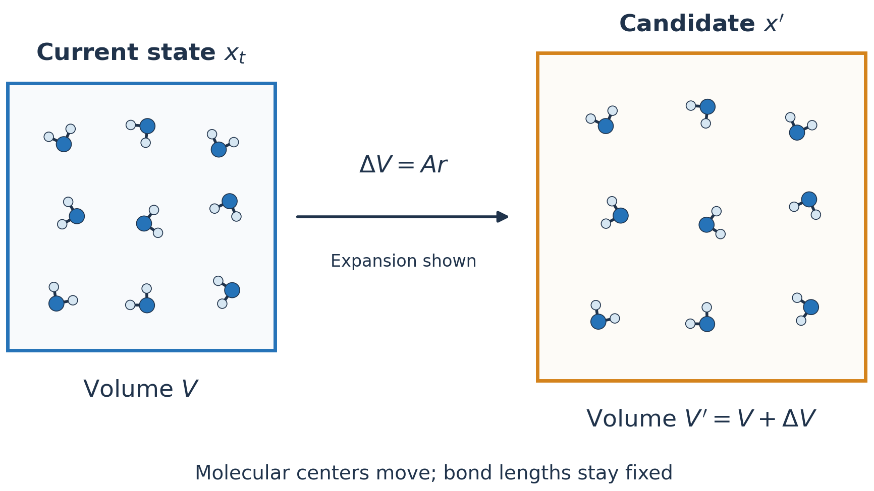
- Generate a candidate $x'$ from distribution $g(x' | x_t)$
- $\Delta V = A r$, $A$ is a scale factor, $r$ is a uniform random number [-1,1]
- Box is scaled to achieve $\Delta V$ - molecules are moved farther apart to be less dense (or closer to be more dense)
- Calculate a weight function
- $\Delta W=\Delta E+P\Delta V-Nk_{B}T \text{ln}\left(\frac{V+\Delta V}{V}\right)$
- $\Delta E$ is change in potential energy due to box resizing
- Accept or reject
- If $\Delta W \le 0$
- Leave the box resized
- Else $\Delta W \gt 0$
- Keep box resized with probability $e^{-\frac{\Delta W }{ k_B T}}$
- If $\Delta W \le 0$
import py3Dmol
import openmm
from openmm.app import *
from openmm.unit import *
from openmm.openmm import *

modeller = Modeller(Topology(),[])
forcefield = ForceField('amber14-all.xml', 'amber14/tip3p.xml')
modeller.addSolvent(forcefield,boxSize=(5,5,5),ionicStrength=.01*molar)

system = forcefield.createSystem(modeller.topology,  nonbondedMethod=PME,constraints=HBonds)
barostat = MonteCarloBarostat(1*atmospheres, 300*kelvin, 250)
system.addForce(barostat)

simulation = Simulation(modeller.topology, system, LangevinIntegrator(300*kelvin,1/picosecond,2*femtosecond))
simulation.context.setPositions(modeller.positions)
simulation.minimizeEnergy()
simulation.reporters.append(StateDataReporter('outputp.txt', 1, step=True, volume=True,
        potentialEnergy=True, kineticEnergy=True, totalEnergy=True, temperature=True))


simulation.step(25000)
import pandas as pd
datap = pd.read_csv('outputp.txt')
datap['Box Volume (nm^3)'].plot()
plt.legend(); plt.xlabel('Frame');

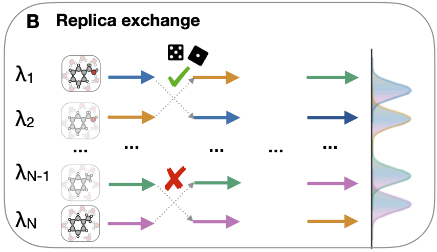
Hamiltonian Replica Exchange
We want our sampled conformations to overlap between alchemical states, so let's allow our trajectories to move between alchemical states to speed up mixing.
If we're careful, we can do this and still sample the correct (Boltzmann) distributions of each state.
Metropolis Criteria
We don't want to arbitrarily move between alchemical states. We will only swap conformations between states if they are reasonably likely in the new state.
Consider two alchemical states $i, j$ with corresponding conformations $r^N_i$, $r^N_j$. Then we will swap with probability:
$$\Large \begin{split}P_{\text{accept}}(i, r^N_i, j, r^N_j) &= \text{min}\left( 1, \frac{ e^{-\left[u_i(r^N_j) + u_j(r^N_i)\right]}}{e^{-\left[u_i(r^N_i) + u_j(r^N_j)\right]}} \right) \\ &= \text{min}\left( 1, e^\left[-\Delta u_{ij}(r^N_i) - \Delta u_{ji}(r^N_j)\right] \right) \end{split}$$ Given enough sampling, this will converge to the correct distributions while enhancing mixing (the different alchemical states will have overlapping conformations).
Gibbs sampling considers swapping between all alchemical states at once (not just neighbors).
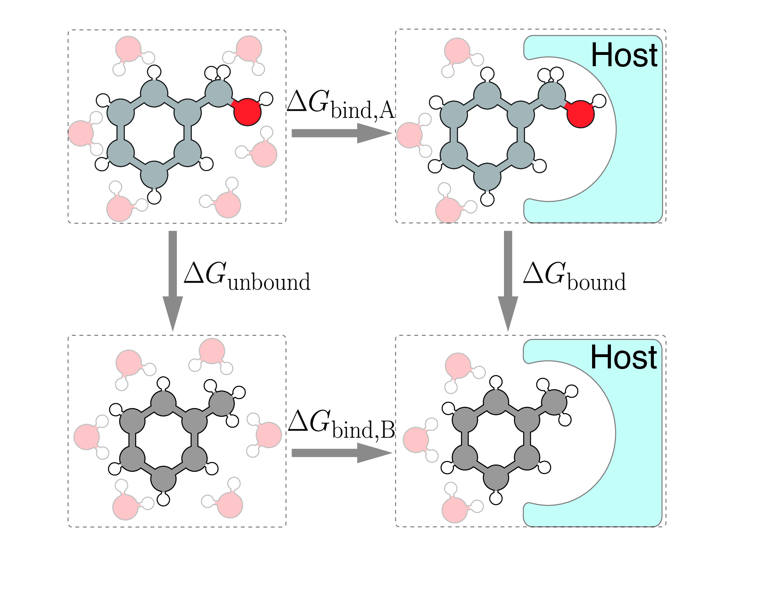
Relative Free Energy Calculations (FEP)
Instead of removing the ligand, convert the ligand to a different ligand to get a $\Delta\Delta G$
FEP Topologies
Need to identify the atoms that should stay the same - the maximum common substructure (MCS).
Rings require special treatment.
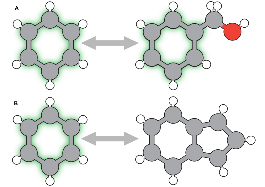
FEP Topologies
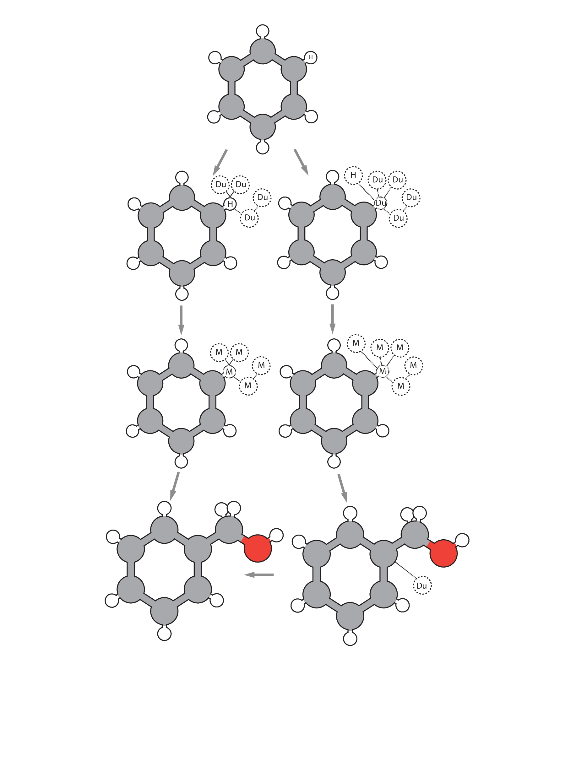
Two methods for dealing with changing atoms:
A single topology (left side): atoms interconvert between molecules (e.g., a hydrogen can become a carbon).
A dual topology (right side): atoms interconvert to "dummy" atoms.
Choice largely depends on software package, although fewer dummy atoms is assumed to be better.
Which topology has fewer dummy atoms?
What do we do with $\lambda$?
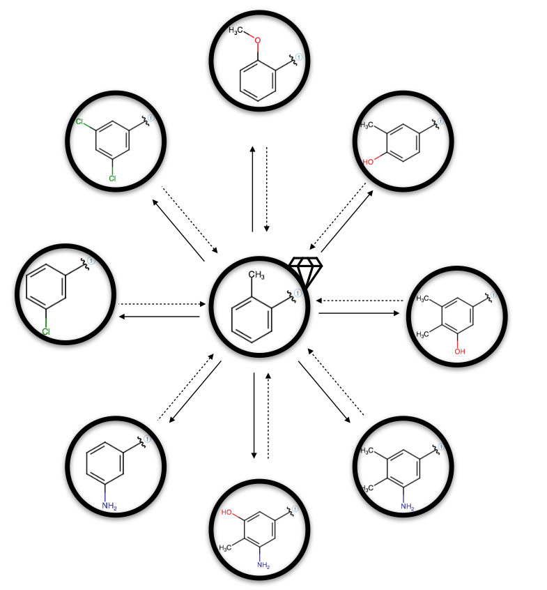
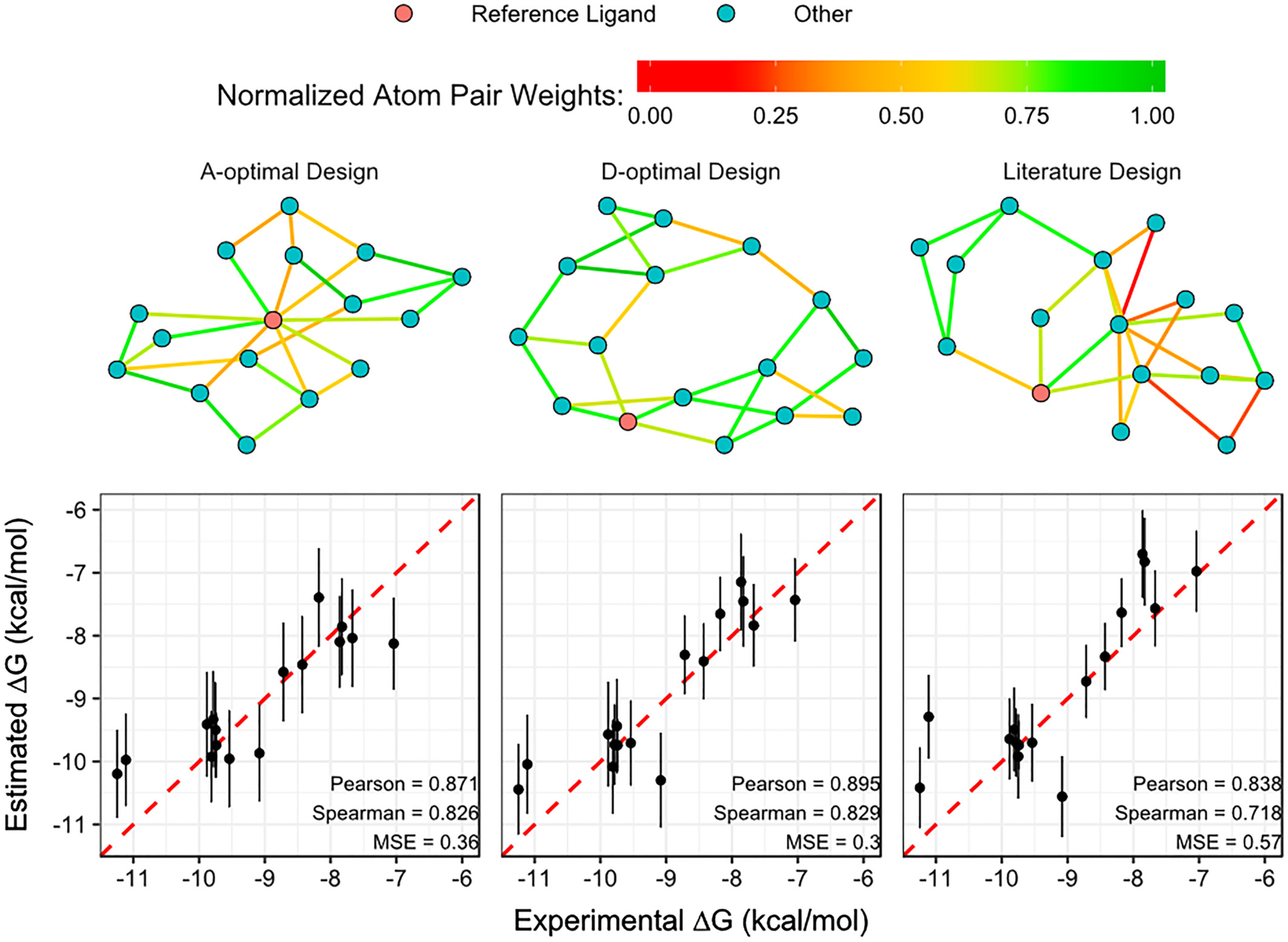
FEP Networks
FEP is usually used during lead optimization to evaluate possible (small) modifications to a lead compound.
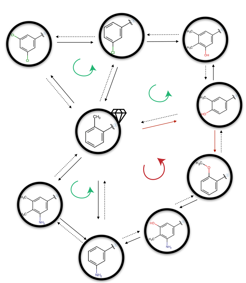
FEP Networks
Where things get exciting is when we perform FEP calculations not only with respect to the known ligand, but between putative ligands.
This lets us compute cycle closure error.
How would you exploit this if you were the computational biologist in charge of running FEP calculations at a large pharmaceutical with a large computing budget (assume the dominant source of error is insufficient sampling)?
Key Points
- FEP: Free Energy Perturbation
- Important: Need correct binding pose
- Can estimate free energy differences along alchemical paths
- Need overlapping samples: can increase with replica-exchange
- Need to compute $\Delta f$: MBAR, TI
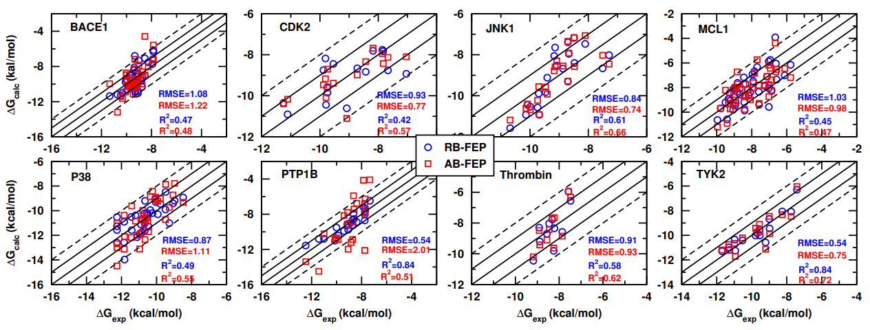
- ABFE vs RBFE
- FEP networks
- cycle closure
- MCMC
- samples equilibrium distributions with relative probabilities
- useful moves can be nonphysical