Deep Learning and Molecular Representations

10/14/2026

print view

%%html
<script src="https://bits.csb.pitt.edu/preamble.js"></script>

Exam 1

Neurons

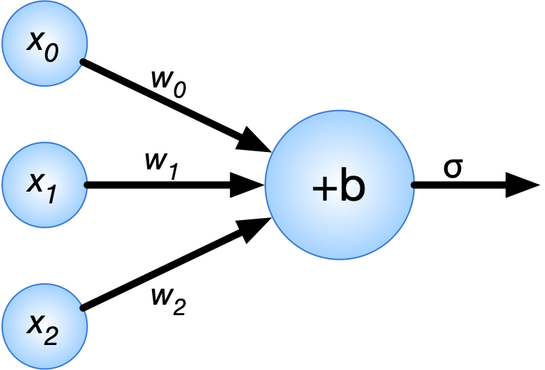
The output of a linear combination of the inputs (with weights $w$ and bias $b$) set the output to the result of a nonlinear activation function $\sigma$

$$\Large \mathrm{output} = \sigma(w\cdot x + b)$$

Activation Functions: Sigmoid (Logistic)

$$\sigma(x) = \frac{1}{1+e^{-ax}}$$

plt.plot(x, 1/(1+np.exp(-x)),linewidth=4,clip_on=False,label='a=1');plt.plot(x, 1/(1+np.exp(-2*x)),linewidth=2,clip_on=False,label='a=2');plt.plot(x, 1/(1+np.exp(-.5*x)),linewidth=2,clip_on=False,label='a=0.5'); plt.xlabel(r"preactivation $z$"); plt.ylabel(r"activation $\sigma(z)$"); plt.legend();

Activation Functions: Rectified Linear Unit (ReLU)

$$\sigma(x) = \max(0,x)$$

plt.plot(x,x*(x > 0),clip_on=False,linewidth=4); plt.xlabel(r"preactivation $z$"); plt.ylabel(r"activation $\sigma(z)$");

Networks

Terminology alert: networks of neurons are sometimes called multilayer perceptrons

Networks

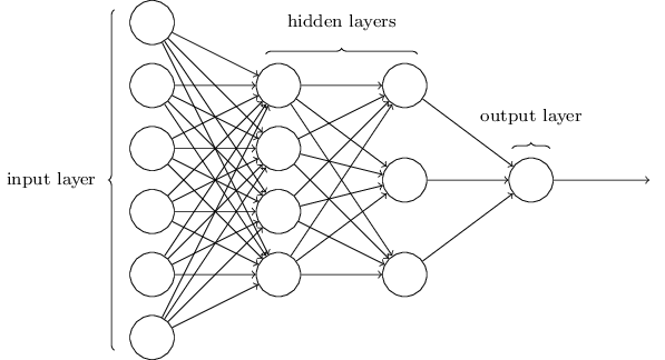
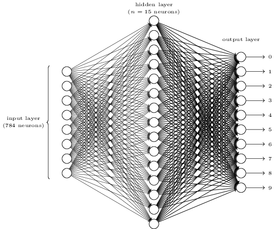The number of input neurons corresponds to the number of features.

The number of output neurons corresponds to the number of label classes. For binary classification, it is common to have two output nodes.

Layers are typically fully connected.

Neural Networks

The universal approximation theorem says that, if some reasonable assumptions are made, a feedforward neural network with a finite number of nodes can approximate any continuous function to within a given error $\epsilon$ over a bounded input domain.

The theorem says nothing about the design (number of nodes/layers) of such a network.

The theorem says nothing about the learnability of the weights of such a network.

These are open theoretical questions.

Given a network design, how are we going to learn weights for the neurons?

Stochastic Gradient Descent

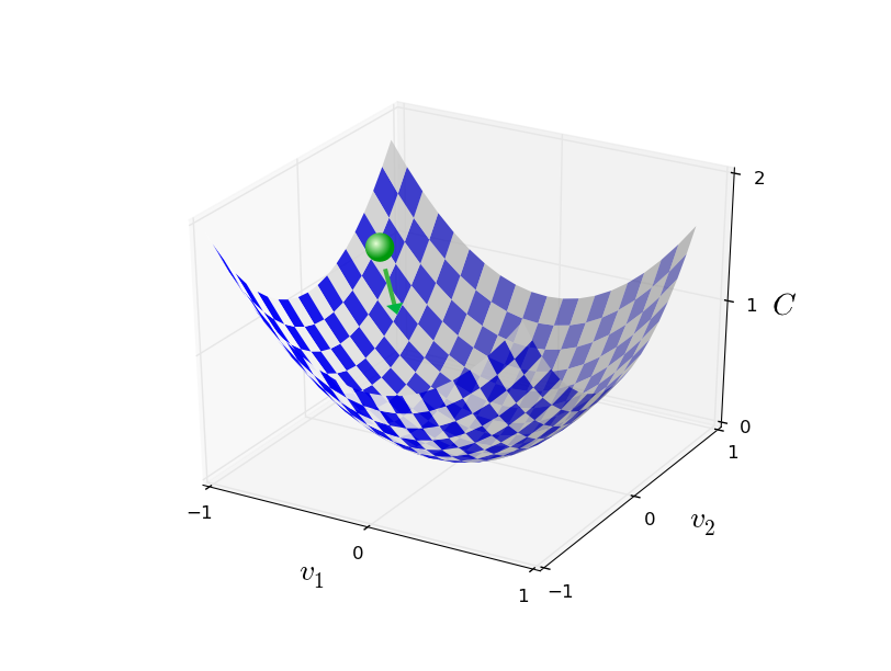
Randomly select $m$ training examples $X_j$ and compute the gradient of the loss function ($L$). Each random selection of $m$ examples is called a batch. Update weights and biases with a given learning rate $\eta$. $$\Large w_k' = w_k-\frac{\eta}{m}\sum_j^m \frac{\partial L_{X_j}}{\partial w_k}$$ $$\Large b_l' = b_l-\frac{\eta}{m} \sum_j^m \frac{\partial L_{X_j}}{\partial b_l} $$

• batch: set of $m$ examples that are used to calculate gradient
• step: one gradient update
• epoch: sufficient steps that the entire training set has been covered

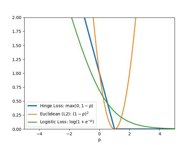
Common loss functions: logistic, hinge, cross entropy, Euclidean

%%html
<div id="bpopt" style="width: 500px"></div>
<script>
$('head').append('<link rel="stylesheet" href="https://bits.csb.pitt.edu/asker.js/themes/asker.default.css" />');

    var divid = '#bpopt';
	jQuery(divid).asker({
	    id: divid,
	    question: "Will SGD (eventually) converge to a global optimum?",
		answers: ["Yes","No","Depends"],
        server: "https://bits.csb.pitt.edu/asker.js/example/asker.cgi",
		charter: chartmaker})
    
$(".jp-InputArea .o:contains(html)").closest('.jp-InputArea').hide();


</script>

Loss Functions

x = 1 is a correct prediction

Example

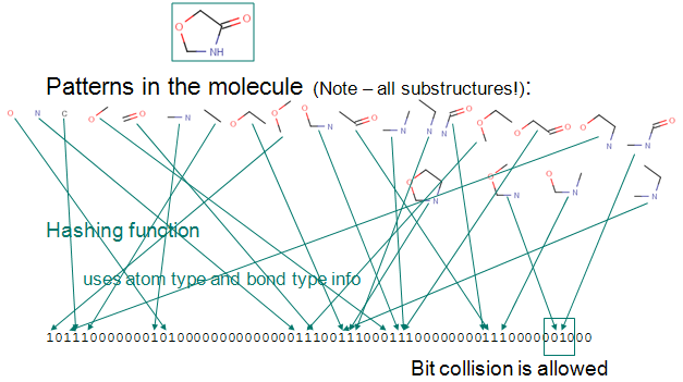
Cheminformatics data. Predict if something is a kinase inhibitor based on molecular fingerprint.

import numpy as np
import sklearn
from sklearn.model_selection import KFold

data = np.genfromtxt('compounds.fp',comments=None)
X = data[:,2:]
Y = data[:,1]

X

array([[0., 0., 0., ..., 0., 0., 0.],
       [0., 0., 0., ..., 0., 0., 0.],
       [0., 0., 0., ..., 0., 0., 0.],
       ...,
       [0., 0., 0., ..., 0., 0., 0.],
       [0., 0., 0., ..., 0., 0., 0.],
       [0., 0., 0., ..., 0., 0., 0.]])

Y

array([1., 1., 1., ..., 0., 0., 0.])

X.shape,Y.shape,sum(Y)

((10600, 2048), (10600,), 5300.0)

Cross Validation

In cross validation we train on a portion of the data and test on the remainder to evaluate the generalizability of our model.

K-Fold Cross Validation

• split data into k parts, or folds
• train k models, each using a different set of k-1 folds
• evaluate on held out set

If k == n, called leave-one-out cross validation.

%%html
<div id="kfold1struct" style="width: 500px"></div>
<script>
$('head').append('<link rel="stylesheet" href="https://bits.csb.pitt.edu/asker.js/themes/asker.default.css" />');

    var divid = '#kfold1struct';
	jQuery(divid).asker({
	    id: divid,
	    question: "In 5-fold cross validation, on average, how many times is a given data point included in a test set?",
		answers: ["1","2","2.5","4","5"],
        server: "https://bits.csb.pitt.edu/asker.js/example/asker.cgi",
		charter: chartmaker})
    
$(".jp-InputArea .o:contains(html)").closest('.jp-InputArea').hide();


</script>

Generalization: What Is Really New?

A validation set should represent the predictions you want.

Random splits can put closely related examples in training and validation, making performance look better than it will be on genuinely new data.

• Proteins — sequence similarity split

  • Cluster related sequences and keep each cluster in one split.
  • Tests generalization to unfamiliar sequences rather than close homologs.

• Small molecules — scaffold split

  • Keep compounds with the same core scaffold in one split.
  • Tests generalization to new chemical series rather than close analogs.
  • Different scaffolds can still be chemically similar—check similarity across splits.

Prevent leakage: keep duplicates and related measurements together;use validation for model selection and an untouched test set for final evaluation.

Ask: Could this validation example have a near-copy in training? Does this split match how the model will be used?

kf = KFold(n_splits=3,shuffle=True)
(train, test) = list(kf.split(data))[0]
Xtrain = X[train]
Ytrain = Y[train]
Xtest = X[test]
Ytest = Y[test]

Xtrain.shape,Xtest.shape

((7066, 2048), (3534, 2048))

from sklearn.neural_network import MLPClassifier
from sklearn import metrics
mlp = MLPClassifier()
mlp.fit(Xtrain,Ytrain)

MLPClassifier()

In a Jupyter environment, please rerun this cell to show the HTML representation or trust the notebook.
On GitHub, the HTML representation is unable to render, please try loading this page with nbviewer.org.

plt.plot(mlp.loss_curve_); plt.xlabel('Epoch'); plt.ylabel('Loss');

print("Test on Train Accuracy",metrics.accuracy_score(Ytrain,mlp.predict(Xtrain)))
print("Held out Test Accuracy",metrics.accuracy_score(Ytest,mlp.predict(Xtest)))

Test on Train Accuracy 1.0
Held out Test Accuracy 0.898981324278438

Effect of learning rate

for lr in [0.0001,0.001,0.01,0.1]:
    mlp = MLPClassifier(learning_rate_init=lr,max_iter=200)
    mlp.fit(Xtrain,Ytrain)
    plt.plot(mlp.loss_curve_,label=f'lr={lr}')
plt.xlabel('Iteration'); plt.ylabel('Loss'); plt.legend(loc='best');

Let's Play!

http://playground.tensorflow.org/

Neural Network Architectures

Convolutional Neural Networks

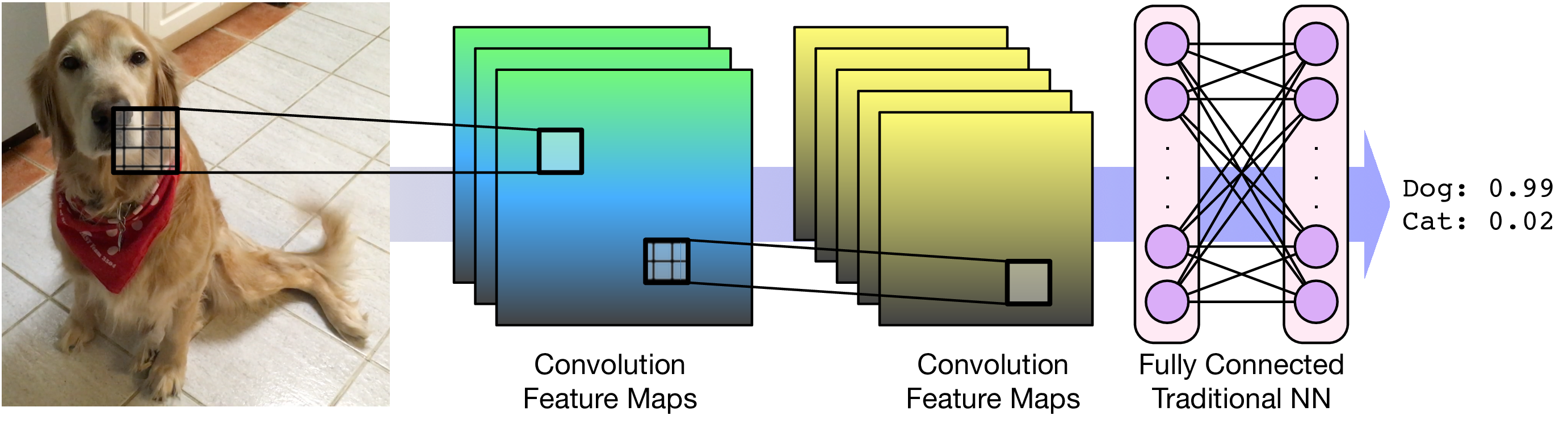
For spatial data (e.g. images). Learn local functions of the input called convolution kernels.

1D Convolution

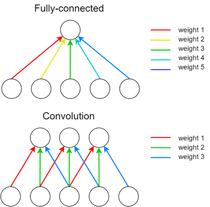A single kernel is applied across the input. For each output feature map there is a single set of weights.

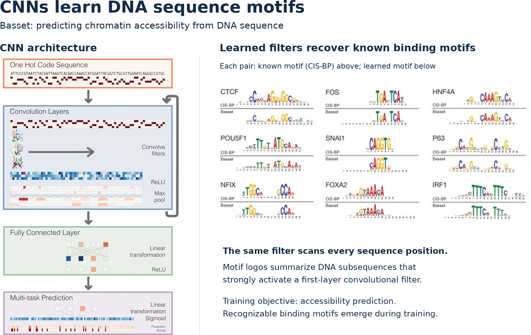
Kelley DR, Snoek J, Rinn JL. Basset: learning the regulatory code of the accessible genome with deep convolutional neural networks. Genome Research 26:990–999 (2016). doi:10.1101/gr.200535.115. Figures 1 and 3B.

Convolution Kernels

The convolution kernel is represented by an $k$x$k$ matrix where the target pixel is in the center.

The output of the filter is the sum of the products of the matrix elements with the corresponding pixels.

Examples (from Wikipedia:

Identity	Blur	Edge Detection

from PIL import Image, ImageFilter
dog = Image.open('imgs/ollygrey.png')
f = plt.figure(figsize=(12,6))
f.add_subplot(1, 2, 1)
plt.imshow(np.array(dog),cmap = cm.Greys_r) 
f.add_subplot(1, 2, 2)
plt.imshow(np.array(dog.filter(ImageFilter.FIND_EDGES)), cmap=cm.Greys_r)
print(ImageFilter.FIND_EDGES.filterargs)

((3, 3), 1, 0, (-1, -1, -1, -1, 8, -1, -1, -1, -1))

Feature Maps

We can think of a kernel as identifying a feature in an image and the resulting image as a feature map that has high values (white) where the feature is present and low values (black) elsewhere.

Feature maps retain the spatial relationship between features present in the original image.

Each feature map is called a channel. For color images, the input starts with 3 channels. Successive layers will have an output channel for each kernel.

Graph Convolutional Neural Networks

Instead of learning a function on a regular grid of neighbors, learn a function on the neighborhood of a node in a graph.

$$h_i = \frac{1}{\deg(i)}\sum_{j \in \mathcal{N}_i} \mathbf{W}x_j$$

Source

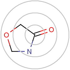
"Convolutional Networks on Graphs for Learning Molecular Fingerprints"

Uses graph convolutions for molecular property prediction.

https://arxiv.org/abs/1509.09292

Transformers

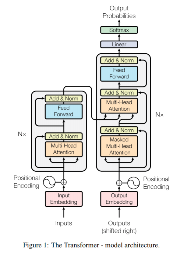
Attention Is All You Need: https://arxiv.org/abs/1706.03762

http://jalammar.github.io/illustrated-transformer/

Context is learned via self-attention

Self-Attention

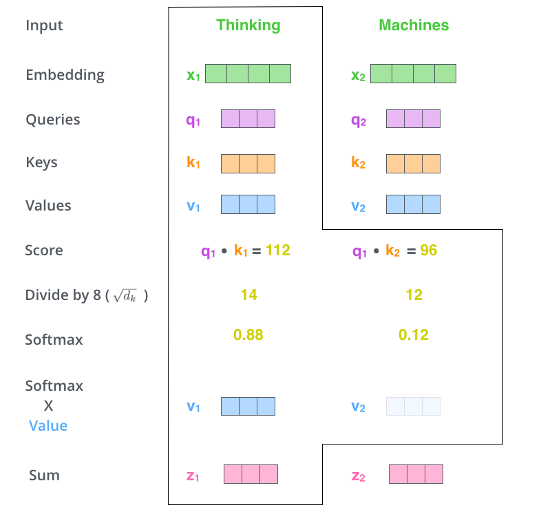
• Have a collection of N objects (e.g. words in a sentence, atoms in a molecule) represented as vectors
• Want to generate N representations of these objects that is context aware
• For each object generate
  • A query: what this object is looking for in other objects
  • A key: what the object provides to other objects
  • A value: what the contribution of this object should be if key matches query
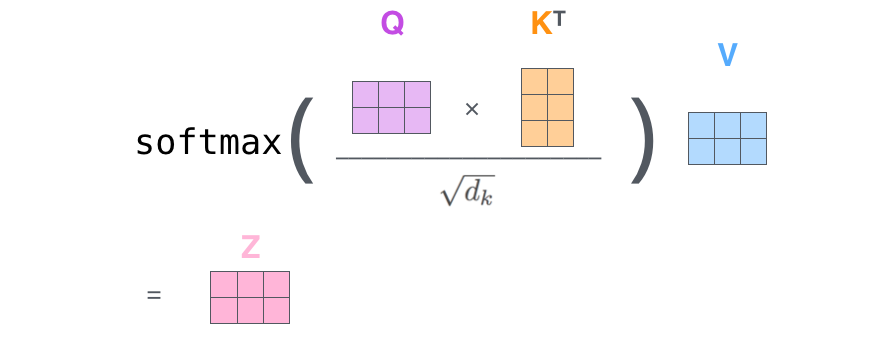
• Each of these is a different learned linear function (weight matrix + optional bias) of the input object

$$Q=XW_Q,\quad K=XW_K,\quad V=XW_V,\qquad \mathrm{Attention}(X)=\mathrm{softmax}_{\mathrm{row}}(QK^T/\sqrt{d_k})V$$

Self-Attention

http://jalammar.github.io/illustrated-transformer/

(Not Self) Attention Mechanism

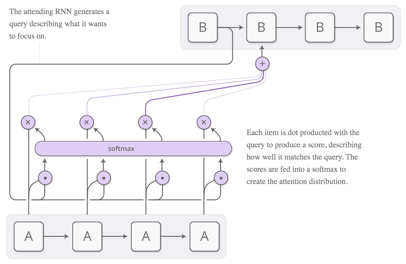
https://distill.pub/2016/augmented-rnns/#attentional-ex2

https://arxiv.org/pdf/1409.0473.pdf

Attention Weights

Bahdanau et al., 2015

Molecular Representations

Representation	Encodes	Main limitation / choice
Fingerprint	Chosen graph neighborhoods	Hash collisions; typically no explicit conformer
SMILES tokens	Serialized graph, optionally stereo	Multiple strings per molecule; tokenization matters
Molecular graph	Atom/bond connectivity and features	Geometry absent unless supplied
3D point set / geometric graph	Atom types and coordinates	Conformer, neighbor rule, and symmetry choices
Voxel grid	Spatial atom-density channels	Resolution, memory, and orientation dependence

"Molecular de-novo design through deep reinforcement learning"

https://jcheminf.biomedcentral.com/articles/10.1186/s13321-017-0235-x#Fig9

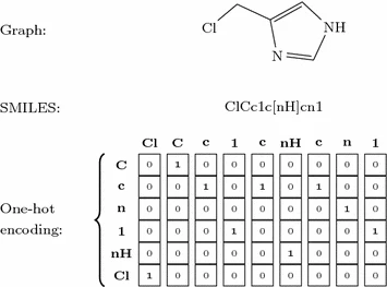
Note tokenization of SMILES

"Molecular de-novo design through deep reinforcement learning"

https://jcheminf.biomedcentral.com/articles/10.1186/s13321-017-0235-x#Fig9

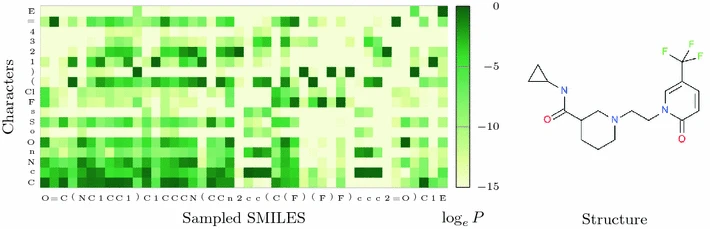
How the model "thinks". Uses GRUs.

"Molecule Attention Transformer"

Consistently out-performs graph convolutions in their evaluations.

Maziarka Ł, Majchrowski D, Danel T, Gaiński P, Tabor J, Podolak I, Morkisz P, Jastrzębski S. Relative molecule self-attention transformer. Journal of Cheminformatics. 2024 Jan 3;16(1):3. Paper

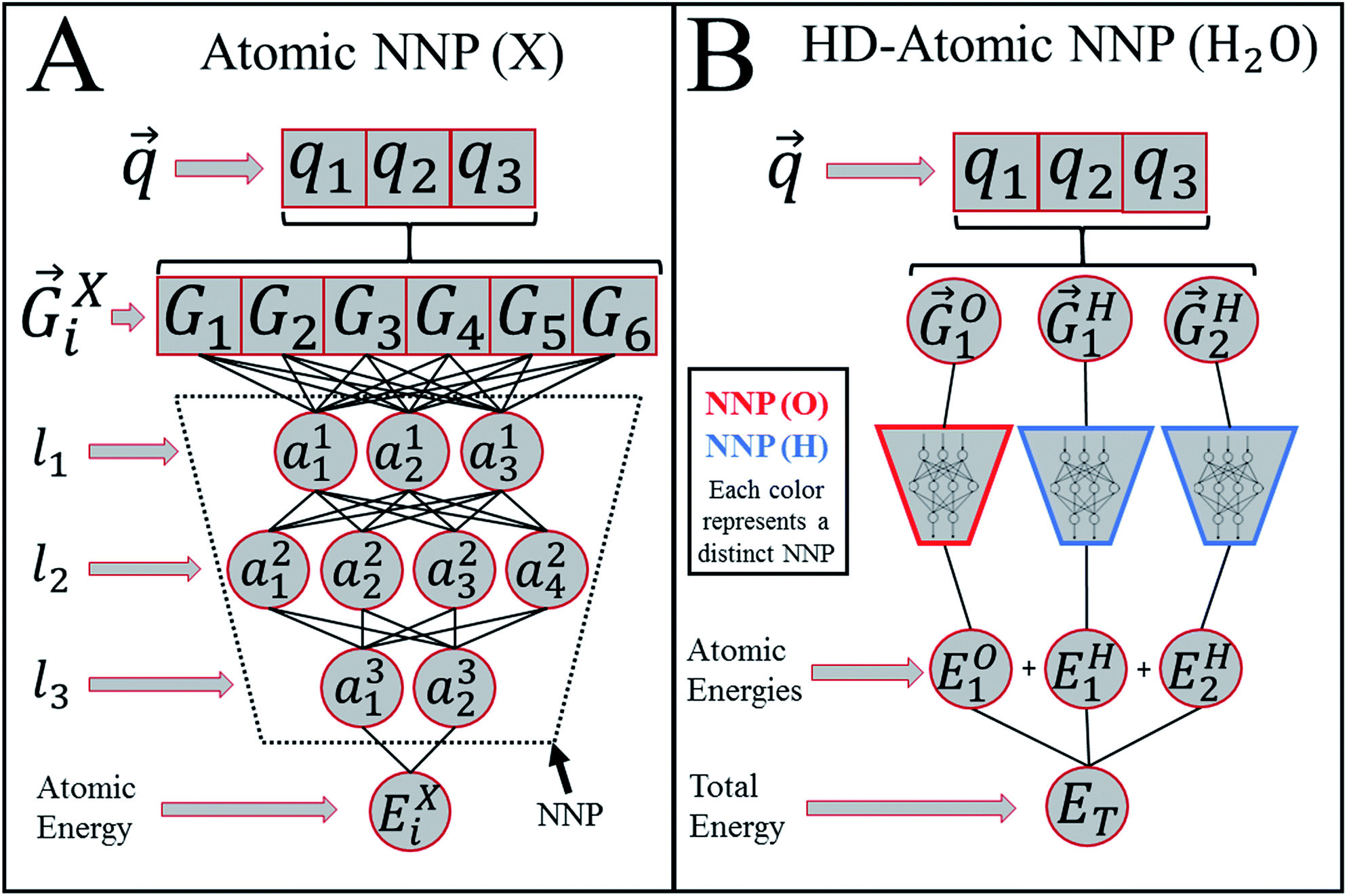
Atomic Environment Vectors

https://pubs.rsc.org/en/content/articlelanding/2017/SC/C6SC05720A

Each atom has its local environment summarized into a vector (this can get complicated)

• bond distances, angles, atom types, etc
• only "sees" atoms within cutoff distance
• result is sum of individual atomic contributions

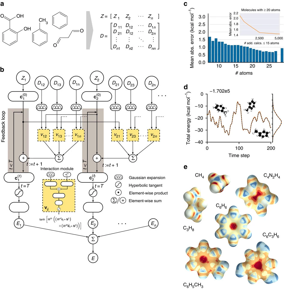
"Quantum-chemical insights from deep tensor neural networks"

https://www.nature.com/articles/ncomms13890

MACE: Learning Molecular Energies and Forces

• Higher-order message passing combines information from several neighbors within a local atomic environment.
• Equivariant features retain directional information; the network predicts an invariant total energy:

$$E_\theta(\mathbf r)=\sum_i E_{\theta,i}, \qquad \mathbf F_i=-\nabla_{\mathbf r_i}E_\theta(\mathbf r)$$

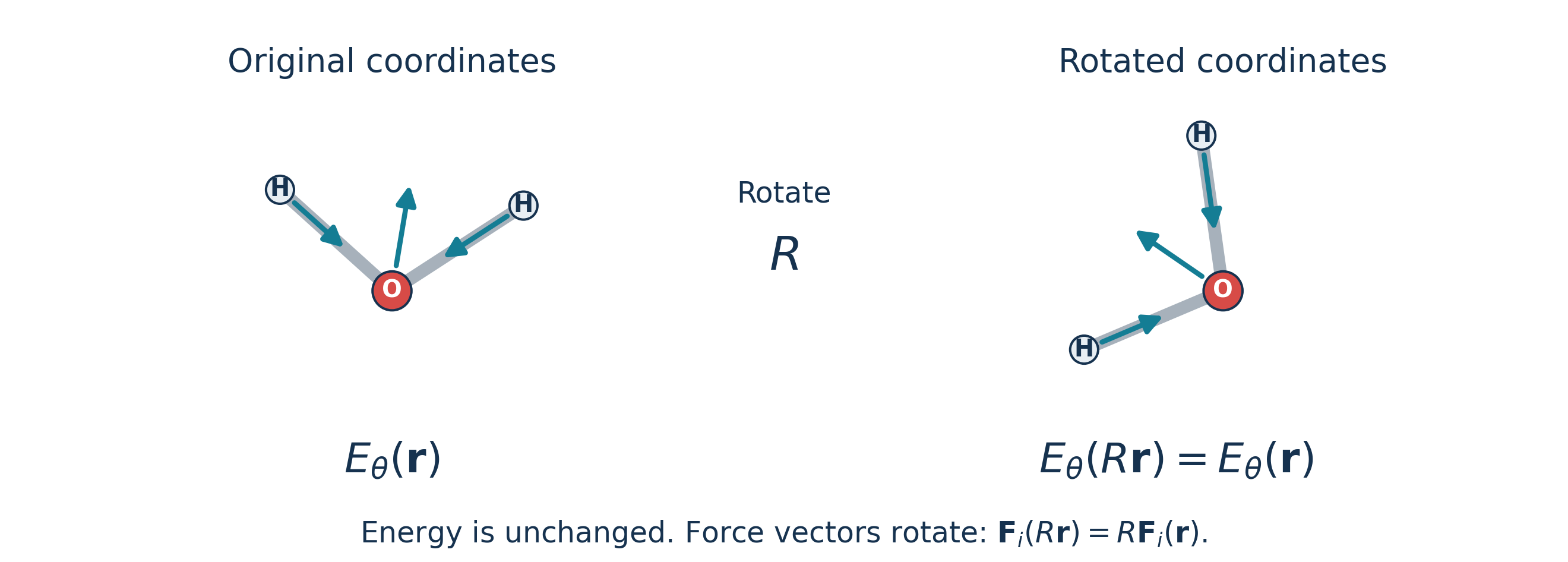
Train on reference energies and forces; use the learned forces in molecular dynamics.

Batatia et al. MACE: Higher Order Equivariant Message Passing Neural Networks for Fast and Accurate Force Fields. NeurIPS (2022). Paper.

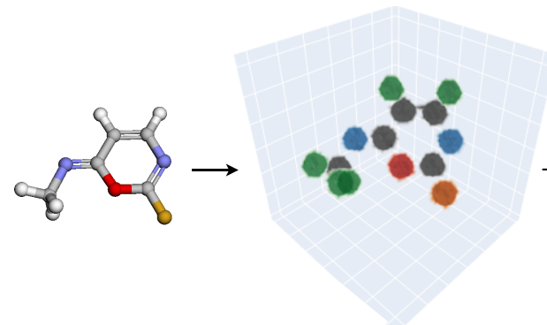
Grids

Protein–Ligand Scoring with Convolutional Neural Networks

3D molecule generation by denoising voxel grid

Basically a 3D picture with atom types instead of red/green/blue.

EGNN: Equivariant Graph Neural Networks

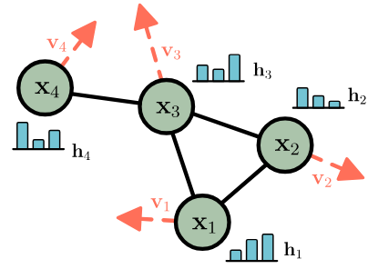
$$\begin{align*} \mathbf{m}_{ij} &= \phi_e\left(\mathbf{h}_i^l,\mathbf{h}_j^l, ||\mathbf{x}_i^l - \mathbf{x}_j^l||^2, a_{ij}\right) \\ \mathbf{v}_i^{l+1} &= \phi_v\left( \mathbf{h}_i^l \right)\mathbf{v}_i^{\mathrm{init}} + C \sum_{j \ne i} \left( \mathbf{x}_i^l - \mathbf{x}_j^l \right) \phi_x \left( \mathbf{m}_{ij} \right) \\ \mathbf{x}_i^{l+1} &= \mathbf{x}_i^l + \mathbf{v}_i^{l+1} \\ \mathbf{m}_i &= \sum_{j \ne i} \mathbf{m}_{ij} \\ \mathbf{h}_i^{l+1} &= \phi_h(\mathbf{h}_i^l,\mathbf{m}_i) \end{align*}$$

Satorras, V. G., Hoogeboom, E., & Welling, M. (2021). E(n) Equivariant Graph Neural Networks. ICML. See §3.2 and Appendix B for the velocity extension.

Invariance

We will get the same output even if the input is transformed (in a certain way).

$$f(T(x)) = f(x)$$

= dog

= dog

Equivariance

The output will be transformed the same way as the input if the input is transformed (in a certain way).

$$f(T(x)) = T'(f(x))$$

= dog

dog =

At the highest level we (probably) want our network to be invariant to rotations and translations.

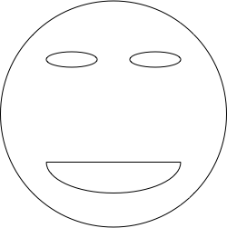= dog

= dog

%%html
<div id="rotationinvariance" style="width: 500px"></div>
<script>
$('head').append('<link rel="stylesheet" href="https://bits.csb.pitt.edu/asker.js/themes/asker.default.css" />');

var divid = '#rotationinvariance';
jQuery(divid).asker({
    id: divid,
    question: "For which output would we NOT want rotation invariance.",
    answers: [
        "Its potential energy",
        "Its molecular weight",
        "The force vector acting on each atom",
        "Its aqueous solubility"
    ],
    server: "https://bits.csb.pitt.edu/asker.js/example/asker.cgi",
    charter: chartmaker
});

$(".jp-InputArea .o:contains(html)").closest('.jp-InputArea').hide();
</script>

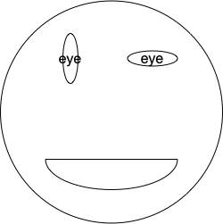
But for lower level filters (features) invariance may make things worse.

=>

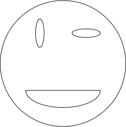With equivariant filters, features with different transformations applied can be seen to be different.

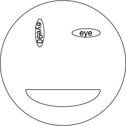
Key Takeaways

• Neural networks fit data

  • Need to test on withheld test set to evaluate generalizability
  • Test set should avoid information leakage

• Network Architectures

  • Convolutional Neural Networks - learn functions on spatially local space
  • Graph Convolutional Neural Networks - learn functions on local neighborhood of nodes
  • Attention (Transformers) - learns query/key/value functions whose outputs are combined to identify what to pay attention to

• Molecular Representations

• 2D: fingerprints, SMILES, graphs

• 3D Graphs

  • Complete (full-connected), e.g. point cloud
  • Nearest neighbor

• Grids (volumetric)

And now for something completely different the same

Score-based Generative Models

https://yang-song.net/blog/2021/score/