%%html
<script src="https://bits.csb.pitt.edu/preamble.js"></script>
<style>:root {--jp-cell-prompt-width: 32px}
img[alt="Pulling a ligand from the binding site"] {width:540px;max-width:100%;max-height:280px;object-fit:contain;}
img[alt="Ligand exit direction and six pulling-force traces"] {float:right;width:40%;max-width:400px;margin:0 0 .45em .7em;}
img[alt="PLP-removal PMFs for E. coli and human SHMT"] {width:590px;max-height:365px;max-width:100%;object-fit:contain;background:white;}
img[alt="Cysteine-distance profiles across runs with and without frataxin"] {width:675px;max-height:380px;max-width:100%;object-fit:contain;background:white;}
.es-fep-movie {display:block;max-width:100%;max-height:390px;margin:.2em auto;object-fit:contain;}
img[alt="Physical and aMD double-well potentials with the boost threshold"],
img[alt="Harmonic GaMD boost falls to zero at the threshold"],
img[alt="Two conditional boost distributions with equal means and variances but different high-boost tails"],
img[alt="Locations and relative PMF values of five reported alanine dipeptide minima"] {display:block; width:760px; max-width:100%; max-height:315px; height:auto; object-fit:contain; margin:.25em auto;}
img[alt="Original potential and boosted potentials for four values of alpha"] {width:450px;max-width:100%;height:auto;}
</style>
<style>
.es-review-band {font-family:system-ui,sans-serif; clear:both;}
.reveal .jp-RenderedHTMLCommon:has(.es-review-band), .reveal .text_cell_render:has(.es-review-band) {font-size:0.82em; line-height:1.24;}
.es-ref {display:block; text-align:right; margin-top:.6em;}
.es-poll [hidden] {display:none !important;}
.es-poll li {margin-bottom:.36em;}
.es-poll .asker-answer {text-align:left;}
.reveal .jp-CodeCell:has(.es-poll) .jp-InputArea, .reveal .code_cell:has(.es-poll) .input, .reveal .jp-CodeCell:has(.es-poll) .jp-OutputPrompt {display:none;}
img[alt="Two basins A and B separated by an energy barrier"] {float:right;max-width:100%;height:auto;}
img[alt="Examples of geometric and learned collective variables"] {width:500px;max-width:100%;height:auto;}
img[alt="Accepted and rejected MCMC moves and the sampled histogram"] {float:right;max-width:100%;height:auto;}
img[alt="Replica overlap for total potential energy in REMD and effective exchange energy in REST1"] {float:right;width:400px;max-width:100%;height:auto;}
img[alt="Structures and residue fluctuations in wild-type and mutant M-crystallins"] {float:right;width:400px;max-width:100%;height:auto;}
img[alt="Patel and Hosur article about self-association sites in M-crystallin"] {width:300px;max-width:100%;height:auto;}
img[alt="Folded M-crystallin and two unfolded conformations of the triple mutant"] {width:300px;max-width:100%;height:auto;}
img[alt="Weighted trajectories exploring a free-energy barrier"] {float:right; width:300px;max-width:100%;height:auto;}
img[alt="Propagation and resampling of weighted walkers across three bins"] {width:800px;max-width:100%;height:auto;}
img[alt="p53 end-to-end distance in angstroms over 40 weighted ensemble iterations"] {width:49%;max-width:520px;height:auto;}
img[alt="Harmonic umbrella windows placed across a double-well profile"] {float:right;width:300px;max-width:100%;height:auto;}
img[alt="Restraint centers and overlapping distributions from neighboring umbrella windows"] {width:550px;max-width:100%;height:auto;}
img[alt="Animation of a peptide pulled from an amyloid protofibril"] {width:400px;max-width:100%;height:auto;}
img[alt="Force on the harmonic pulling spring over 500 ps"] {width:600px;max-width:100%;height:auto;}
img[alt="Aβ42 dissociation PMF and sampled distance histograms for individual windows"] {width:400px;max-width:100%;height:auto;}
</style>
The problem

We are most interested in biological processes that have longer timescales than we can easily simulate.
- Ligand binding/unbinding
- Protein folding/unfolding
- Complex formation/aggregation
- Large conformational changes
We need to be able to sample rare events.
Approaches
Simplify the topology to make it faster to simulate
- Coarse-graining
- Implicit solvent
Use multiple simulations to better sample
- Weighted Ensemble
- Replica Exchange
- Umbrella Sampling
Change the energy function to make rare events more likely
- Steered MD
- Umbrella Sampling
- Accelerated MD
- Metadynamics
many, many, many more...
Another categorization
Collective variable free
- Coarse-graining, implicit solvent, MCMC, Replica Exchange, aMD, GaMD
Collective variable required
- Weighted Ensemble, Steered MD, Umbrella Sampling, Metadynamics...
What is a collective variable (CV)?
A collective variable is a function of the coordinates, such as ligand–pocket distance or the number of binding-site contacts.
It is typically a lower dimensional representation of the system that we want to sample along: $z^M = \xi(r^N), M \ll N$
A useful reaction coordinate (or preogress coordinate) also tracks progress between the states of interest.
What are examples of collective variables for ligand unbinding?

Replica Exchange: Using multiple simulations to sample rare events
Recall from this picture that energy barries get smaller at higher temperature.


Replica Exchange Metropolis-Hastings
Both replicas use the same potential energy function $U$. Let $r_i$ and $r_j$ denote the coordinates of all $N$ atoms in the two conformations. Their potential energies are $U(r_i)$ and $U(r_j)$, and their initial temperatures are $T_i$ and $T_j$, respectively.
How does the joint Boltzmann weight change if we swap the temperature assignments? For a symmetric swap proposal, divide the swapped weight by the current weight. Let $\Delta U = U(r_j) - U(r_i)$.
$$\Large p_{\mathrm{acc}} = \min \left( 1, \frac{ \exp \left( -\frac{U(r_j)}{k_BT_i} - \frac{U(r_i)}{k_BT_j} \right) }{ \exp \left( -\frac{U(r_i)}{k_BT_i} - \frac{U(r_j)}{k_BT_j} \right) } \right) \\ \Large = \min \left( 1, e^{-\Delta U \left( \frac{1}{k_BT_i} - \frac{1}{k_BT_j} \right)} \right) $$
On an accepted swap, each conformation keeps its coordinates. Rescale its velocities for its new temperature by multiplying by $\sqrt{T_{\mathrm{new}}/T_{\mathrm{old}}}$.
Problem
Higher temperature $\rightarrow$ Higher average energy (distribution shift)
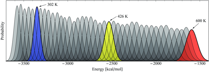
What is the problem here?
Problem: Larger systems require more replicas/smaller temperature differences
Number of replicas needed scales $\sqrt{N_\mathrm{df}}$ where $N_\mathrm{df}$ is the number of degrees of freedom in the system derivation.
Consider the decomposition of the energy into protein/water components:
$$E = E_p + E_w + E_{pw}$$
Where are most of the degrees of freedom?
Replica Exchange with Solute Tempering (REST)
Let $T_0$ be the target temperature and $T_m$ the temperature of replica $m$. Scale the protein ($p$), water ($w$), and protein–water ($pw$) energy terms as follows.
$$\Large U_m = U_p + \frac{T_m}{T_0}U_w + \frac{T_m+T_0}{2T_0}U_{pw}$$
At $T_m = T_0$, we recover the original potential. As $T_m$ increases, the water–water term grows by $T_m/T_0$. This exactly offsets the higher temperature in its Boltzmann factor, so the water–water term cancels from the swap ratio.
This is Hamiltonian replica exchange because each replica has a different potential energy function. Suppose replica $m$ initially holds conformation $r_i^N$ and replica $n$ holds conformation $r_j^N$. To exchange them, compare the swapped weight with the current weight.
$$\Large p_{\mathrm{acc}} = \min \left( 1, \frac{ \exp \left( -\frac{U_m(r_j^N)}{k_BT_m} - \frac{U_n(r_i^N)}{k_BT_n} \right) }{ \exp \left( -\frac{U_m(r_i^N)}{k_BT_m} - \frac{U_n(r_j^N)}{k_BT_n} \right) } \right) $$

REST2
Instead of "cooling" water, "heat" the protein. All replicas are run at same temperature, but potential energy of protein is scaled to be "hotter":
$$U_m = \frac{T_0}{T_m} U_p + \sqrt{\frac{T_0}{T_m}}U_{pw} + U_{ww}$$
This is claimed to increase protein conformational sampling.


Weighted Ensemble: Using multiple simulations to sample rare events

Bin configuration space along collective variables (CVs)
- Bins can adapt or be redefined
Run multiple weighted trajectories per bin
- Split and merge to maintain target walker count per occupied bin
Propagate trajectory weights to preserve unbiased statistics
Compute observables — equilibrium from weighted averages, rates from steady-state fluxes
Weighted Ensemble


Steered Molecular Dynamics
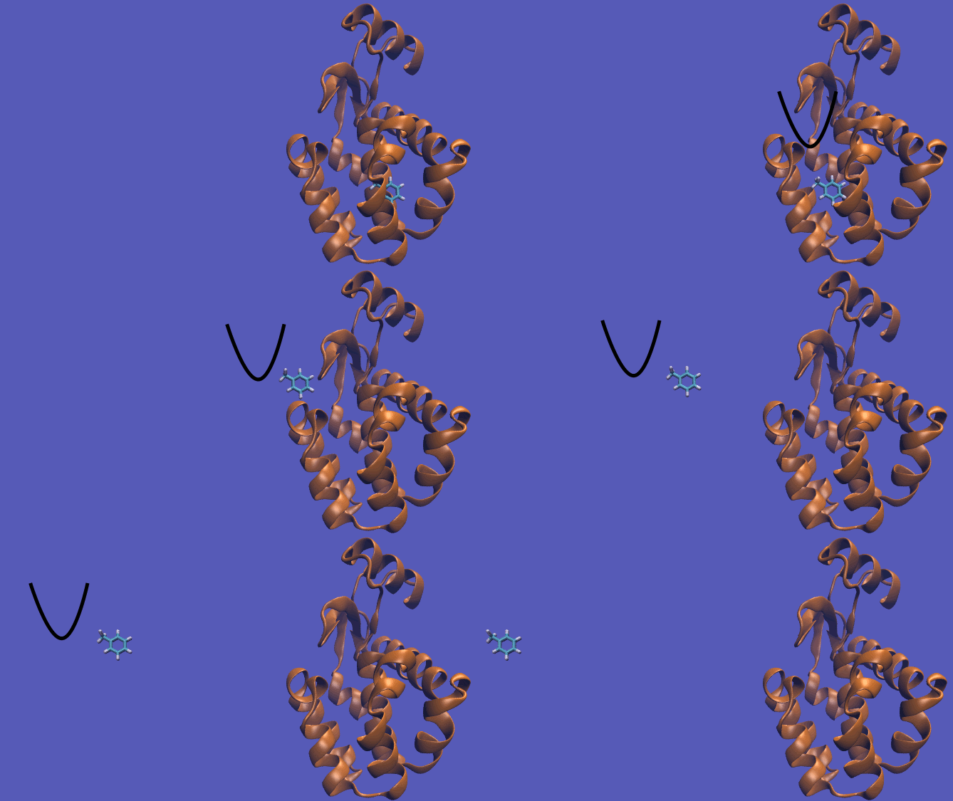
How can we watch a ligand leave its binding pocket on an MD timescale?
Attach a virtual spring to the ligand along a pulling coordinate $s$. Move the center of the spring, $\lambda(t)$, away from the pocket at constant speed $v$.
$$\Large U_{\mathrm{pull}}(s,t) = \frac{1}{2} k \left( s - \lambda(t) \right)^2 \qquad \lambda(t) = \lambda_0 + vt$$
How much work does it take to pull out a ligand?
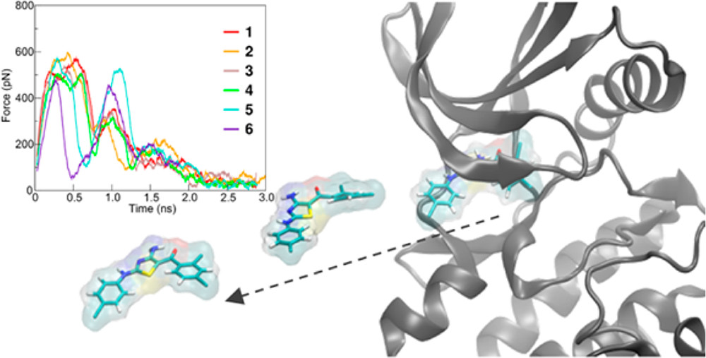
Patel et al. pulled inhibitors out of cyclin-dependent kinase 5 (CDK5). The arrow shows the pulling direction. The inset shows how the force varies during six pulls.
The peak force tells us when the ligand resists most strongly. The work depends on the entire pull. At constant pulling speed $v$,
$$\Large W = \int f_{\mathrm{pull}} \, d\lambda = v \int_0^\tau f_{\mathrm{pull}}(t) \, dt$$
Let $s(t)$ be the ligand’s position along the pulling direction and $\lambda(t)$ the position of the spring center along that same direction. We move the spring center from $\lambda_0$ to $\lambda_1$ in time $\tau$ at constant speed $v = (\lambda_1-\lambda_0)/\tau$.
For a spring of stiffness $k$, the signed pulling force is $f_{\mathrm{pull}}(t) = k[\lambda(t)-s(t)]$. The work $W$ done on the system during one pull is
$$\Large W = \int_{\lambda_0}^{\lambda_1} f_{\mathrm{pull}} \, d\lambda = v \int_0^\tau f_{\mathrm{pull}}(t) \, dt$$
Here $d\lambda = v\,dt$ is the distance the spring center moves during a time interval $dt$. On the force–time plot, multiply the signed area under one trace by $v$ to get the work for that pull.
Free Energy is Related to Work
We move the spring the same way in every pull, yet each pull requires a different amount of work. What is the relationship between the free energy and the average work?
The work required to move a system from state A to state B is
$$\Large \Delta F \le \langle W \rangle $$
The Jarzynski equality states that:
$$\Large \newcommand{\expect}[1]{\left\langle{#1}\right\rangle} e^{-\Delta F/k_\mathrm{B}T} = \expect{e^{-W/k_\mathrm{B}T}}$$
Case Study: SHMT

Case Study: Frataxin
v = py3Dmol.view(width=800,query='6nzu',style={'cartoon': {'colorscheme':'chainHetatm'}}); v.addStyle({'resi':381},'stick'); v.setStyle({'hetflag':True},'stick'); v.setStyle({'bonds':0},'sphere'); v.show();
3Dmol.js failed to load for some reason. Please check your browser console for error messages.
Steered MD Example: Frataxin
Steered MD Example: Frataxin


Umbrella Sampling
We need a collective variable $\xi$ (reaction coordinate) that we divide into $N$ bins indexed by $i$.
We also need starting structures at each $\xi_i$.
We add a harmonic constraint on the collective variable in each bin: $$U^i(r^N) = U(r^N) + \frac{1}{2}k_i(\xi_{r_N} - \xi_i)^2$$
How can we get the starting structures??


Recall: Potential of Mean Force
The PMF is the free energy surface along the reaction coordinate. $$\Large e^{-\mathrm{PMF}(\xi)/k_B T} \propto \rho^u(\xi) $$
Here $\rho^u$ is the unbiased probability, without our harmonic potential (what we actually care about).
$$\Large \rho^u_i(\xi) = \frac{\int \delta\left(\xi-{\xi}(\mathbf{r}^N)\right) e^{-U(\mathbf{r}^N)/k_B T} d\mathbf{r}^N}{\int e^{-U(\mathbf{r}^N)/k_B T} d\mathbf{r}^N}$$
What we've computed is the biased probability, $\rho^b_i$.
Unbiasing
Let $$\Large \omega_i(\xi_{r_N}) = k_i(\xi_{r_N} - \xi_i)^2$$
Show that $$\Large \rho^u_i(\xi) = \rho^b_i(\xi) e^{\omega_i(\xi)/k_\mathrm{B}T} \langle e^{-\omega_i(\xi_{r^N})} \rangle_{r^N} $$
$$ \rho^u_i(\xi) = \frac{\int \delta\left(\xi-{\xi}(\mathbf{r}^N)\right) e^{-U(\mathbf{r}^N)/k_B T} d\mathbf{r}^N}{\int e^{-U(\mathbf{r}^N)/k_B T} d\mathbf{r}^N}$$
$$ \rho^b_i(\xi) = \frac{\int \delta\left(\xi-{\xi}(\mathbf{r}^N)\right) e^{-\left[ U(\mathbf{r}^N)+\omega({\xi}(\mathbf{r}^N))\right]/k_B T} d\mathbf{r}^N}{\int e^{-\left[ U(\mathbf{r}^N)+\omega({\xi}(\mathbf{r}^N))\right]/k_B T} d\mathbf{r}^N}$$
$$ = e^{-\omega_i(\xi)/k_B T} \frac{\int \delta\left(\xi-{\xi}(\mathbf{r}^N)\right) e^{-U(\mathbf{r}^N)/k_B T} d\mathbf{r}^N}{\int e^{-\left[ U(\mathbf{r}^N)+\omega({\xi}(\mathbf{r}^N))\right]/k_B T} d\mathbf{r}^N}$$
$$e^{-\omega_i(\xi)/k_B T} \frac{\int \delta\left(\xi-{\xi}(\mathbf{r}^N)\right) e^{-U(\mathbf{r}^N)/k_B T} d\mathbf{r}^N}{\int e^{-\left[ U(\mathbf{r}^N)+\omega({\xi}(\mathbf{r}^N))\right]/k_B T} d\mathbf{r}^N} \times\; e^{\omega_i(\xi)/k_B T} \frac{\int e^{-\left[ U(\mathbf{r}^N)+\omega({\xi}(\mathbf{r}^N))\right]/k_B T} d\mathbf{r}^N}{\int e^{-U(\mathbf{r}^N)/k_B T} d\mathbf{r}^N} $$
$$ = \rho^u_i(\xi) $$
Solving for the PMF
The ensemble average over the biasing potential is the free energy difference, $F_i$, between the biased and unbiased state:
$$\Large e^{F_i/k_\mathrm{B}T} = \langle e^{-\omega_i(\xi_{r^N})} \rangle_{r^N}$$
The full PMF depends on all the windows and we must solve self-consistently for all $F_i$. This is a discretized version of MBAR.
Key Idea
We biased the energy potential, ran simulations, and then can unbias the results to get the free energy change.
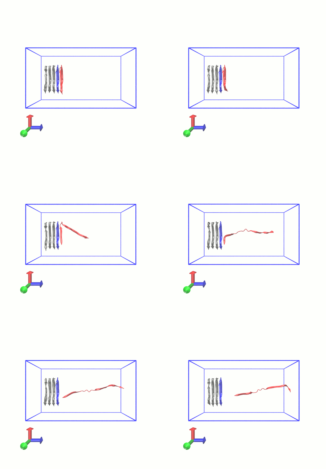
Example (Gromacs Tutorial):

Example (Gromacs Tutorial):

Accelerated Molecular Dynamics
When the energy is below a threshold, $E$, add a boost potential $\Delta U$:
$$U^*(r^N) = \begin{cases} U(r^N) & U(r^N) \ge E\\ U(r^N) + \Delta U(r) & U(r^n) < E \end{cases} $$

Boost Potential
An example: $$ \Delta U(\mathbf{r}) = \frac{(E-U(\mathbf{r}))^2}{\alpha + (E-(U(\mathbf{r}))}$$
The boost potential may be selectively applied to components of the force field (e.g., only nonbonded interactions and torsions).
The boost potential effectively increases the time scale of the simulation when in effect:
$$\Delta t^*_i = \Delta t e^{\Delta U(\mathbf{r})}$$
Removing aMD bias
Suppose half the frames in an accelerated MD trajectory are folded. Does that mean the equilibrium folded population is 50%?
As in umbrella sampling, we undo the bias by weighting each frame. If aMD raised the potential energy of frame $i$ by $\Delta U_i$, its weight is
$$\Large w_i = e^{\Delta U_i/(k_\mathrm{B}T)}$$
A larger boost gives a frame more weight because aMD made that conformation less favorable.
$$\Large P(\mathrm{folded}) \approx \frac{\sum_{i\,\in\,\mathrm{folded}} w_i}{\sum_{\mathrm{all}\ i} w_i}$$
Gaussian accelerated MD uses a harmonic boost
Below $E_{\mathrm{thr}}$, add $\Delta U=\tfrac12 k(E_{\mathrm{thr}}-U)^2$.

With both methods a frame’s weight is (e^{\Delta U/(k_BT)}). In aMD, a few high-boost frames can therefore determine the estimated folded population. GaMD uses the energy fluctuations measured during equilibration to choose one spring constant $k$. It lifts the wells as much as it can while keeping the estimated variation in boost energies below a chosen limit.
Metadynamics
Metadynamics is an adaptive biasing potential approach. Requires collective variable. With some rate, add a bias potential (usually a Gaussian with width and height parameters) at the current collective variable location.
Metadynamics
The potential is a sum of Gaussian kernels deposited along the trajectory in collective variable space
$$\Large U(\vec{s},t) = \sum_{ k \tau < t} W(k \tau) \exp\left( -\sum_{i=1}^{d} \frac{(s_i-s_i(\mathbf{q}(k \tau)))^2}{2\sigma_i^2} \right)$$
$W$ is the simulation height (function of time), $\tau$ is the deposition stride, $\sigma_i$ the width of the Gaussian for $i$th CV, and $s(q)$ defines the collective variables.
BioEmu samples a protein ensemble directly
BioEmu trains a diffusion model on AlphaFold structures, MD ensembles, and experimental folding stabilities. Given a sequence, it generates independent backbone conformations from a learned approximation to the equilibrium ensemble.

Which enhanced sampling method should I use?
| If my goal is… | I would choose… |
|---|---|
| Transition pathways and rates | Weighted ensemble. Define the starting and target states, propagate unbiased dynamics, and estimate the rate from weighted steady-state flux. |
| A PMF along a known coordinate | Umbrella sampling. Place overlapping windows along the coordinate and equilibrate each one. |
| Explore a landscape with a few good CVs | Metadynamics. Bias regions already visited to discover other basins along those CVs. |
| Test a proposed exit route or seed umbrella windows | Steered MD. Pull along that route. The pulling direction and speed influence what you observe. |
| Equilibrium sampling without a clear CV | Replica exchange if I can afford a replica ladder; REST2 if the slow motions are mainly in the solute. |
| Explore without a clear CV using one biased trajectory | aMD or GaMD. Favor GaMD if I need equilibrium populations, and check that the reweighted estimates are reproducible. |
| Rapidly propose protein conformations from sequence | BioEmu. Sample a learned ensemble. The structures can suggest alternative states, but their ordering carries no physical time. |