%%html
<script src="https://bits.csb.pitt.edu/preamble.js"></script>
<style>:root {--jp-cell-prompt-width: 32px}</style>
GNM & ANM: Elastic Network Models
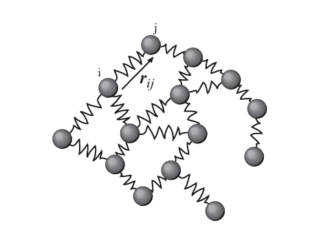
Given a single structure, infer its dynamics by representing it as a bunch of balls connected by springs.
- Each residue becomes a ball
- Residues within a cutoff (e.g. 10Å) are connected with springs
- No conventional molecular energies, just springs
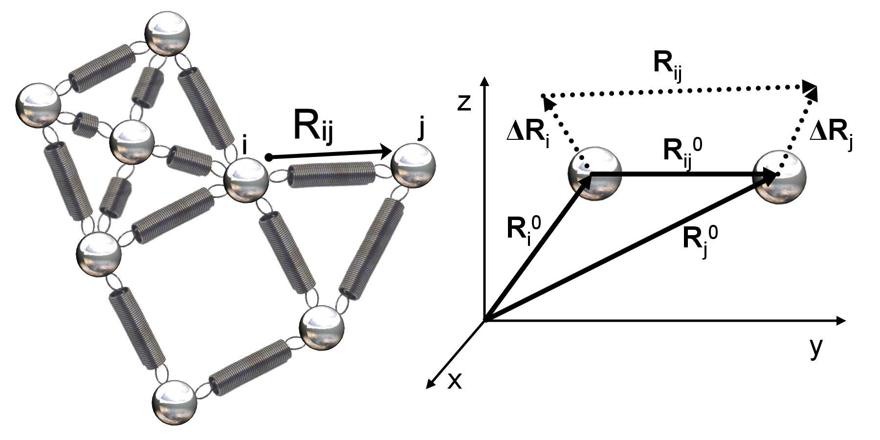
Gaussian Network Model (GNM)
The potential energy of the elastic network is:
$$U_{GNM} = \frac{\gamma}{2}\left[ \sum_{i,j\in \mathrm{edges}} (\Delta R_j-\Delta R_i)^2 \right]= \frac{\gamma}{2}\left[ \sum_{i,j}^{N} \Delta R_i \Gamma_{ij} \Delta R_j\right]$$
where $\Gamma$ is the Kirchhoff matrix, or graph Laplacian, $D-A$:
$$\Gamma_{ij} = \left\{\begin{matrix} -1, & \mbox{if } i \ne j & \mbox{and }R_{ij} \le r_c \\ 0, & \mbox{if } i \ne j & \mbox{and }R_{ij} > r_c \\ -\sum_{j,j \ne i}^{N} \Gamma_{ij}, & \mbox{if } i = j \end{matrix}\right. $$
Gaussian Network Model (GNM)
If we decompose the potential into its Cartesian components:
$$U_{GNM} = \frac{\gamma}{2}\left[ \sum_{i,j}^{N} \Delta R_i \Gamma_{ij} \Delta R_j\right] = \frac{\gamma}{2} [\Delta X^T\Gamma \Delta X + \Delta Y^T\Gamma \Delta Y + \Delta Z^T\Gamma \Delta Z]$$
where $$\Delta X^T = [\Delta X_1, \Delta X_2, \cdots \Delta X_N]$$
and apply the Boltzmann distribution:
$$p(\Delta R)\propto \exp\left\{ -\frac{\gamma}{2 k_B T} \left[\Delta X^T\Gamma \Delta X + \Delta Y^T\Gamma \Delta Y + \Delta Z^T\Gamma \Delta Z\right] \right\}$$
we can see the probability is isotropic:
$$p(\Delta R)=p(\Delta X,\Delta Y,\Delta Z)=p(\Delta X)p(\Delta Y)p(\Delta Z)$$
Gaussian Network Model (GNM)
A multivariate Gaussian distribution: $$\mathcal{N}(\boldsymbol\mu,\, \boldsymbol\Sigma) = \frac{1}{\sqrt{(2\pi)^N |\Sigma|}} \exp\left\{ -\frac{1}{2} (x - \mu)^T \Sigma^{-1} (x - \mu) \right\}$$
If we shoehorn our Boltzmann distribution into the Gaussian form we get: $$p(\Delta X)\propto \exp\left\{ -\frac{\gamma}{2 k_B T} \Delta X^T\Gamma \Delta X \right\}=\exp\left\{ -\frac{1}{2} \left(\Delta X^T\left( \frac{k_B T}{\gamma} \Gamma^{-1} \right)^{-1} \Delta X \right) \right\}$$ $$p(\Delta X ) = \frac{1}{\sqrt{(2\pi)^N \frac{k_B T}{\gamma} |\Gamma^{-1}|}} \exp\left\{ -\frac{1}{2} \left(\Delta X^T\left( \frac{k_B T}{\gamma} \Gamma^{-1} \right)^{-1} \Delta X \right) \right\}$$
where
$$Z_X = \int_{\mathbb R^N} \exp\left\{ -\frac{\gamma}{2 k_B T} \Delta X^T\Gamma \Delta X \right\}d\Delta X = \sqrt{ \left(2\pi \frac{k_B T}{\gamma}\right)^N |\Gamma^{-1}|}$$
Gaussian Network Model (GNM)
Now we have $p(\Delta X)$ we can compute expectations of properties.
$$\langle \Delta X \cdot \Delta X^T \rangle = \int \Delta X \cdot \Delta X^T p(\Delta X)d\Delta X=\frac{k_B T}{\gamma}\Gamma^{-1} $$
(this follows from the generalized Gaussian integral)
Since the probability is isotropic, we can get the overall expectation of fluctuations by multiplying by 3:
$$\langle \Delta R_i^2 \rangle = \frac{3 k_B T}{\gamma}(\Gamma^{-1})_{ii}$$ $$\langle \Delta R_i \cdot \Delta R_j \rangle = \frac{3 k_B T}{\gamma}(\Gamma^{-1})_{ij}$$
Gaussian Network Model (GNM)
Slight problem: $\Gamma$ is not invertible. So we take the pseudoinverse constructed from the eigenvalues/vectors of $\Gamma$.
$$\langle \Delta R_i \cdot \Delta R_j \rangle = \frac{3 k_B T}{\gamma}[U\Lambda^{-1}U^T]_{ij}=\frac{3 k_B T}{\gamma}\sum_{k=1}^{N-1}\lambda_k^{-1} [u_k u_k^T]_{ij}$$
We can decompose fluctuations into the contributions from individual modes ($k$):
$$[\Delta R_i \cdot \Delta R_j]_k = \frac{3 k_B T}{\gamma}\lambda_k^{-1} [u_k]_i [u_k]_j$$
Mode interpretation:
- "Slow" (soft, low frequency, small eigenvalue) modes contribute most to the expected fluctuations. Motions are collective and global
- "Fast" (stiff, high frequency, large eigenvalue) modes describe local, less correlated motions
GNM Example
m = prody.parsePDB('6zio').select('chain A')
%%time
gnm, calpha = prody.calcGNM(m,n_modes='all')
CPU times: user 13.2 ms, sys: 1.83 ms, total: 15.1 ms Wall time: 25 ms
help(prody.calcGNM)
Help on function calcGNM in module prody.dynamics.gnm:
calcGNM(pdb, selstr='calpha', cutoff=10, gamma=1.0, n_modes=20, zeros=False)
Returns a :class:`GNM` instance and atoms used for the calculations.
By default only alpha carbons are considered, but selection string helps
selecting a subset of it. *pdb* can be :class:`.Atomic` instance.
GNM Example
prody.showProtein(m).show()
3Dmol.js failed to load for some reason. Please check your browser console for error messages.
GNM Example
gnm
<GNM: 6zio (170 modes; 171 nodes)>
gnm.getKirchhoff()
array([[ 6., -1., -1., ..., 0., 0., 0.],
[-1., 11., -1., ..., 0., 0., 0.],
[-1., -1., 10., ..., 0., 0., 0.],
...,
[ 0., 0., 0., ..., 7., -1., -1.],
[ 0., 0., 0., ..., -1., 5., -1.],
[ 0., 0., 0., ..., -1., -1., 5.]], shape=(171, 171))
GNM Example
prody.showContactMap(gnm,interactive=False);

GNM Example
prody.showCovarianceMatrix(gnm,interactive=False);

Fluctuations
prody.showSqFlucts(gnm); plt.xticks(range(0,175,25));

Fluctuations (MD)
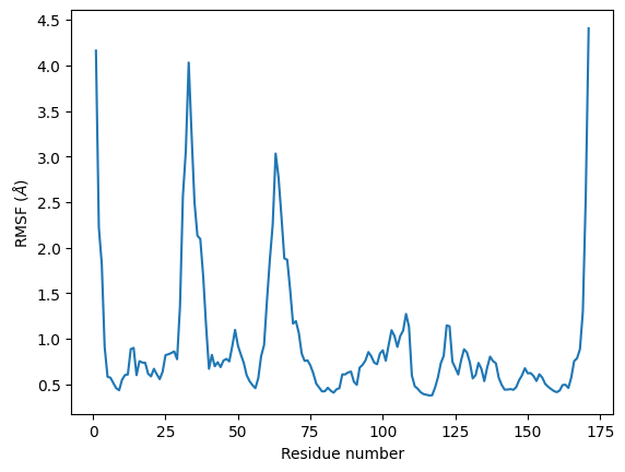
Mode 0 (Slow)
prody.showMode(gnm[0]); ax2 = plt.gca().twinx()
prody.showSqFlucts(gnm[0],color='green'); plt.xticks(range(0,175,25));

prody.showProtein(m,data=gnm[0],width='100%',height='600px').show()
3Dmol.js failed to load for some reason. Please check your browser console for error messages.
prody.showProtein(m,data=prody.calcSqFlucts(gnm[0]),width='100%',height='600px').show()
3Dmol.js failed to load for some reason. Please check your browser console for error messages.
Mode 19 (Fast)
prody.showMode(gnm[19]); ax2 = plt.gca().twinx()
prody.showSqFlucts(gnm[19],color='green'); plt.xticks(range(0,175,25));

prody.showProtein(m,mode=gnm[19],width='100%',height='600px').show()
3Dmol.js failed to load for some reason. Please check your browser console for error messages.
prody.showProtein(m,data=prody.calcSqFlucts(gnm[-1]),width='100%',height='600px').show()
3Dmol.js failed to load for some reason. Please check your browser console for error messages.
Anisotropic Network Model (ANM)
We still have an elastic network with a harmonic potential between connected nodes:
$$U_{ij} = {\gamma\over 2}{( d_{ij} - {d_{ij}}^o)}^2$$ where ${d_{ij}}^o$ is the ideal distance (from the provided structure).
We take second derivatives and evaluate at $d_{ij} = {d_{ij}}^o$:
$${\partial^2 U_{ij}\over\partial x_i \, \partial y_j} = {-\gamma\over d_{ij}^2} {(x_j - x_i)}{(y_j-y_i)} $$
We use these to build a $3N \times 3N$ Hessian matrix formed of $3 \times 3$ blocks $H_{ij}$.
Anisotropic Network Model (ANM)
Hessian
$$H_{ij} = \begin{bmatrix} {\partial^2 U_{ij}\over\partial x_i \, \partial x_j} & {\partial^2 U_{ij}\over\partial x_i \, \partial y_j} & {\partial^2 U_{ij}\over\partial x_i \, \partial z_j} \\ {\partial^2 U_{ij}\over\partial y_i \, \partial x_j} & {\partial^2 U_{ij}\over\partial y_i \, \partial y_j} & {\partial^2 U_{ij}\over\partial y_i \, \partial z_j} \\ {\partial^2 U_{ij} \over\partial z_i \, \partial x_j} & {\partial^2 U_{ij}\over\partial z_i \, \partial y_j} & {\partial^2 U_{ij}\over\partial z_i \, \partial z_j}\end{bmatrix} = {-\gamma\over {d_{ij}}^2} \begin{bmatrix} {(x_j - x_i)(x_j - x_i)} & {(x_j - x_i)(y_j - y_i)} & {(x_j - x_i)(z_j - z_i)} \\ {(y_j - y_i)(x_j - x_i)} & {(y_j - y_i)(y_j - y_i)} & {(y_j - y_i)(z_j - z_i)} \\{(z_j - z_i)(x_j - x_i)} & {(z_j - z_i)(y_j - y_i)} & {(z_j - z_i)(z_j - z_i)} \end{bmatrix} $$
$$H_{ij}=0\quad\text{for noncontacts},\qquad H_{ii}=-\sum_{j\ne i}H_{ij}.$$
We take the eigenvector decomposition $H = U\Lambda U^T$ to get directional modes of motion.
ANM Example
m = prody.parsePDB('2lz3',model=1)
prody.showProtein(m,width='100%').show()
3Dmol.js failed to load for some reason. Please check your browser console for error messages.
ANM Example
anm, calpha = prody.calcANM(m,n_modes='all')
anm
<ANM: 2lz3 (162 modes; 56 nodes)>
help(prody.calcANM)
Help on function calcANM in module prody.dynamics.anm:
calcANM(
pdb,
selstr='calpha',
cutoff=15.0,
gamma=1.0,
n_modes=20,
zeros=False,
title=None
)
Returns an :class:`ANM` instance and atoms used for the calculations.
By default only alpha carbons are considered, but selection string helps
selecting a subset of it. *pdb* can be a PDB code, :class:`.Atomic`
instance, or a Hessian matrix (:class:`~numpy.ndarray`).
ANM Example
anm.getHessian().shape
(168, 168)
anm.getHessian()
array([[ 2.53839681, 1.8851409 , 2.04873159, ..., 0. ,
0. , 0. ],
[ 1.8851409 , 2.61862398, 1.60559669, ..., 0. ,
0. , 0. ],
[ 2.04873159, 1.60559669, 8.84297921, ..., 0. ,
0. , 0. ],
...,
[ 0. , 0. , 0. , ..., 2.49200883,
-2.27617489, 1.47675537],
[ 0. , 0. , 0. , ..., -2.27617489,
3.73316645, -2.40276548],
[ 0. , 0. , 0. , ..., 1.47675537,
-2.40276548, 4.77482471]], shape=(168, 168))
prody.showProtein(m,mode=anm[0],data=prody.calcSqFlucts(anm[0]),anim=False,scale=25,width="100%",height="600px").show()
3Dmol.js failed to load for some reason. Please check your browser console for error messages.
prody.showProtein(m,mode=anm[0],data=prody.calcSqFlucts(anm[0]),anim=True,scale=25,width="100%",height="600px").show()
3Dmol.js failed to load for some reason. Please check your browser console for error messages.
prody.showProtein(m,mode=anm[1],data=prody.calcSqFlucts(anm[1]),anim=True,scale=25,width="100%").show()
3Dmol.js failed to load for some reason. Please check your browser console for error messages.
Comparing ANM to Reality
This structure is actually an NMR structure, so we have an experimental ensemble. Let's compute the PCA of this ensemble to get modes based in reality.
ens = prody.parsePDB('2lz3')
prody.showProtein(ens,width="100%").show()
3Dmol.js failed to load for some reason. Please check your browser console for error messages.
PCA
ensemble = prody.Ensemble(ens.calpha)
print("Before iterpose",ensemble.getRMSDs().mean())
ensemble.iterpose()
print("After iterpose",ensemble.getRMSDs().mean())
Before iterpose 8.253871223076873 After iterpose 0.7246260755875822
pca = prody.PCA()
pca.buildCovariance(ensemble)
pca.calcModes()
PCA
prody.showProjection(ensemble, pca[:2]);

PCA vs ANM
prody.showSqFlucts(pca,label='PCA'); prody.showSqFlucts(anm,label='ANM'); plt.legend();

PCA vs ANM
prody.showOverlapTable(pca[:4], anm[:4],interactive=False);

prody.showProtein(m,data=prody.calcSqFlucts(pca[0]),mode=pca[0].getEigvec(),anim=True,amplitude=25,height="600px",width="100%").show()
3Dmol.js failed to load for some reason. Please check your browser console for error messages.
prody.showProtein(m,data=prody.calcSqFlucts(anm[1]),mode=anm[1],anim=True,amplitude=25,width="100%",height="600px").show()
3Dmol.js failed to load for some reason. Please check your browser console for error messages.
Key Questions
- What reduced representation to use?
- How to represent forces/interactions/energies?
- How to sample/simulate the system?
- What is the goal?
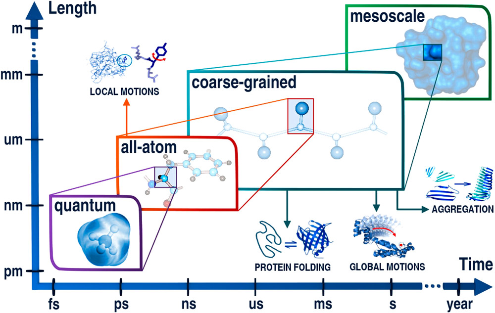
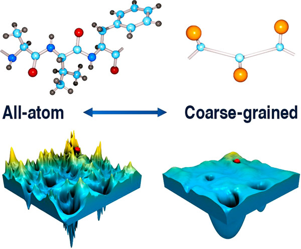
Coarse-Grained Representations
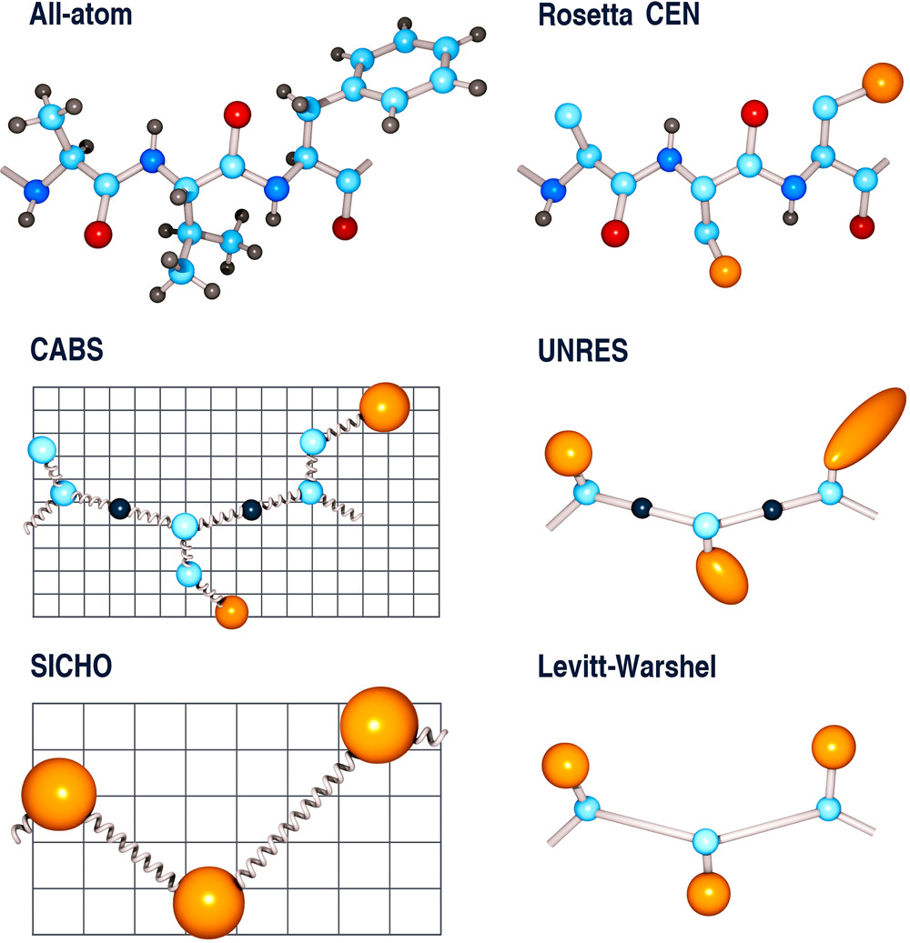
Groups of atoms are represented by interaction sites (beads). Solvent may be implicit or represented by explicit coarse-grained water, depending on the model. Some models further constrain bond lengths, angles, or lattice positions.
MARTINI Model
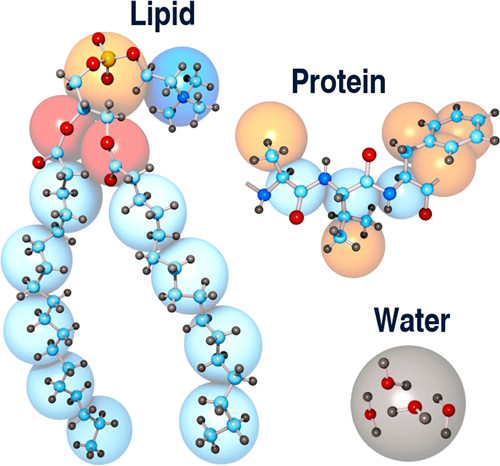
Groups of 2-4 heavy atoms are summarized with a single pseudo atom.
Can be generalized to many different biomolecules.
Very popular for membrane simulations.
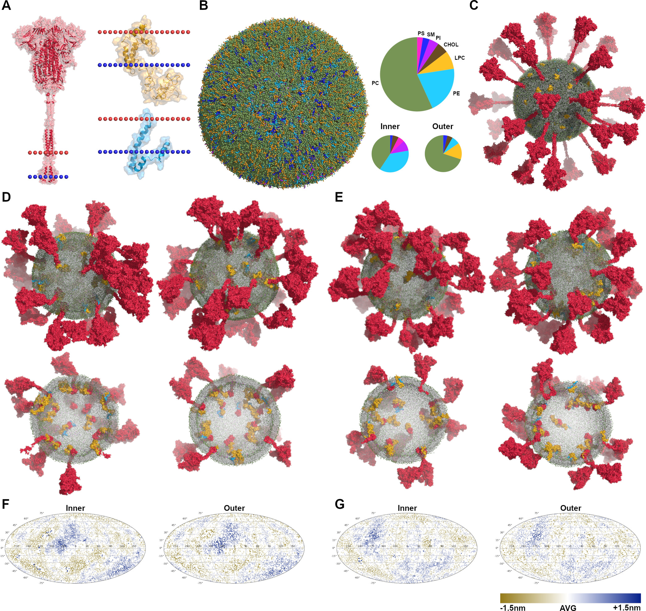
Coarse Grained Interactions
- Force field based: Use similar terms to conventional force field - try to construct an "average" potential for pseudoatoms. "Softer" than all-atom force fields.
- Knowledge based: Construct statistical potentials:
$$ E(X,A) = -\ln \left(P(C\mid X, A)\right) = -\ln \left(\frac{P(X, A\mid C)}{P(X,A)} \right)$$ where $A$ is an amino acid sequence, $X$ is a vector of structural features $X$, and $C$ is a "correct" conformation. $P(X,A\mid C)$ is the distribution of observed "correct" conformations (e.g. the PDB).
- Structure-based: Must know the correct structure. Native contacts have low energy. Usually referred to as Gō potentials.
Gō Potentials

$U(r_i, r_j) =
\begin{cases}
-\varepsilon, & \text{if } (i,j) \in \mathcal{N} \text{ and } \|r_i - r_j\| < r_c \\
0, & \text{otherwise}
\end{cases}$
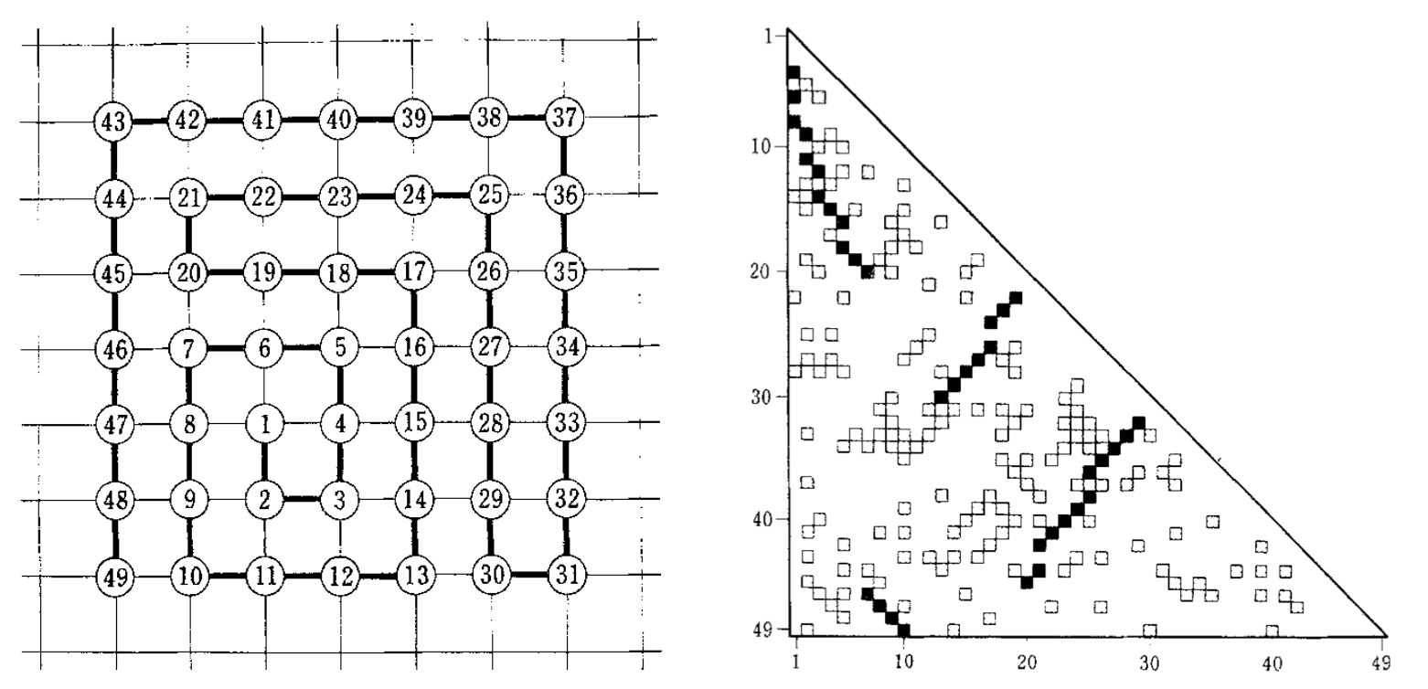
Some implementations use LJ potential for native contacts
Non-native contacts may have repulsion term instead of zero
Can be combined with (parts of) MM force field
Question: How does coarse-graining affect the entropy of the system?
How to sample/simulate the system?
Especially with force field based potentials, can use traditional molecular dynamics (Langevin).
Alternatively, give up on dynamics and use Markov Chain Monte Carlo sampling with Metropolis-Hastings.
If the goal is to identify the lowest energy state (e.g., protein folding) may use search algorithms like genetic algorithms.
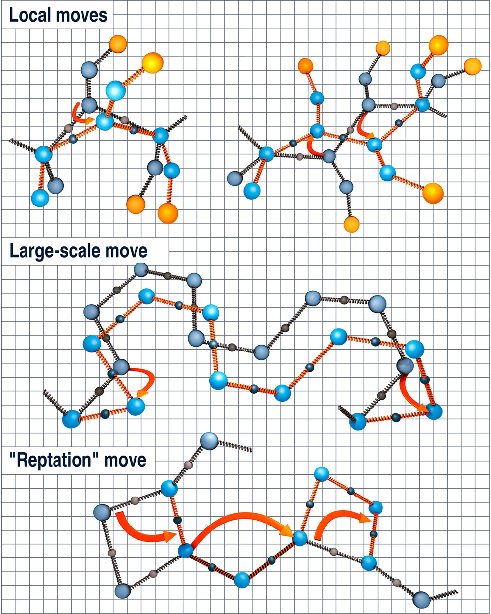
Coarse Grained Move Sets
With fewer interaction sites MCMC can propose larger collective conformational changes. Acceptance still depends on the model's potential, including steric/excluded-volume penalties.
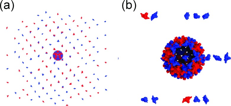
Viral Assembly Example
The entire subunit is treated as a rigid object and Gō potential combined with MCMC and weighted ensemble is used to determine assembly pathways.
Rescuing Coarse Grain Simulation
- Using neural network potentials to achieve better accuracy. Machine learning coarse-grained potentials of protein thermodynamics
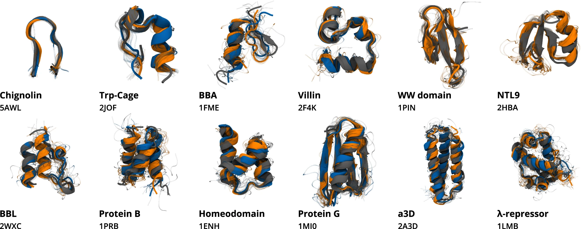
Rescuing Coarse Grain Simulation
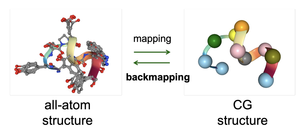
- Learning generative models to restore fine-grain detail to coarse grain simulations (back-mapping). Chemically transferable generative backmapping of coarse-grained proteins
Implicit Solvation
Most of what we simulate in molecular dynamics is water (88% of the atoms in my NRAS simulation were water).
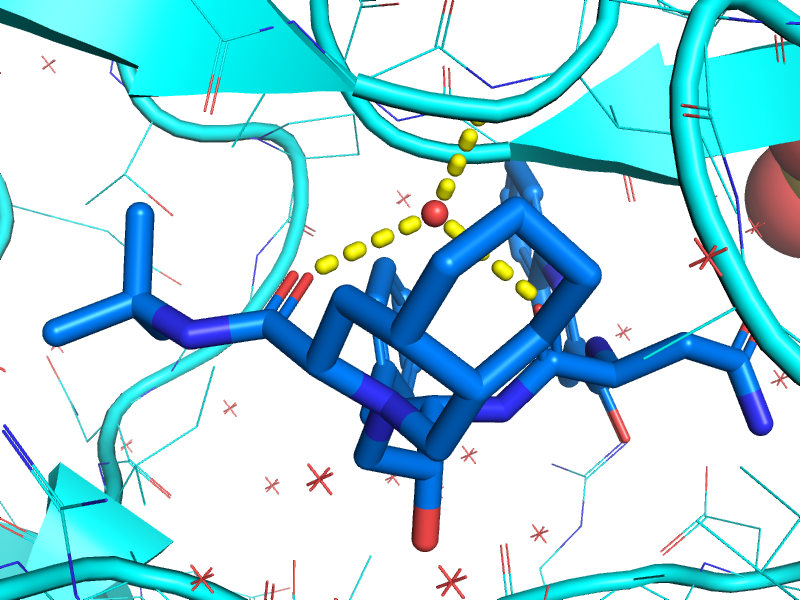 What does this water do?
- Get in the way
- Modify electrostatics
- Nonpolar hydration
- Specific structural role
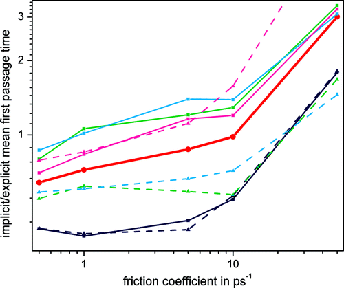
With a Langevin integrator, how can we simulate the motion dampening effects of water (viscosity)?
Friction
$$ m\frac{d^2x}{dt^2}=\mathbf{F}-\gamma m \frac{dx}{dt} +\mathbf{R}$$
Implicit solvent simulations typically increase the friction coefficient (e.g. 10 instead of 1). Or it is left small to accelerate sampling.
Electrostatics
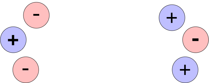
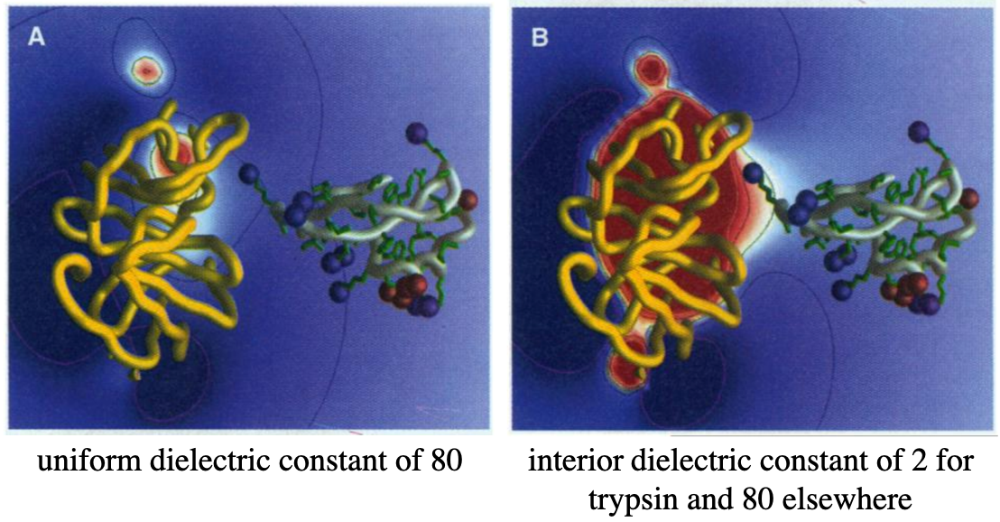
Water, as a strong and mobile dipole, shields charges.
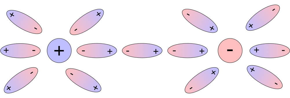
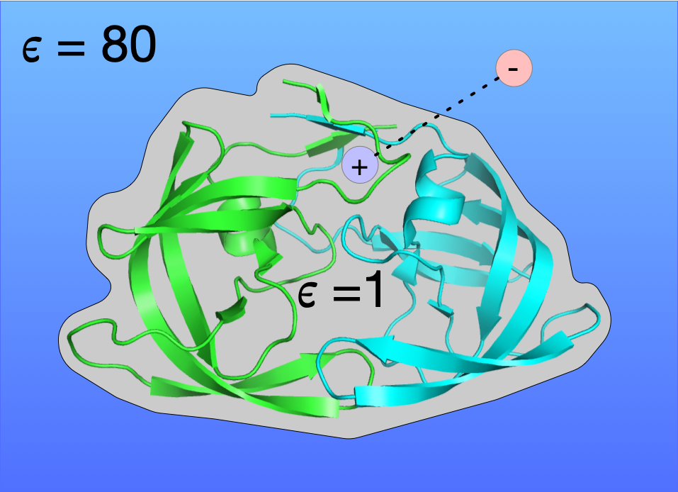
This results in a high dielectric constant $\epsilon$ (~80)
$$U = k\frac{q_i q_j}{\epsilon r_{ij}}$$
Most of the effect is due to the reorganization of the water molecules, not induced polarizability (electrons moving around).
Screening
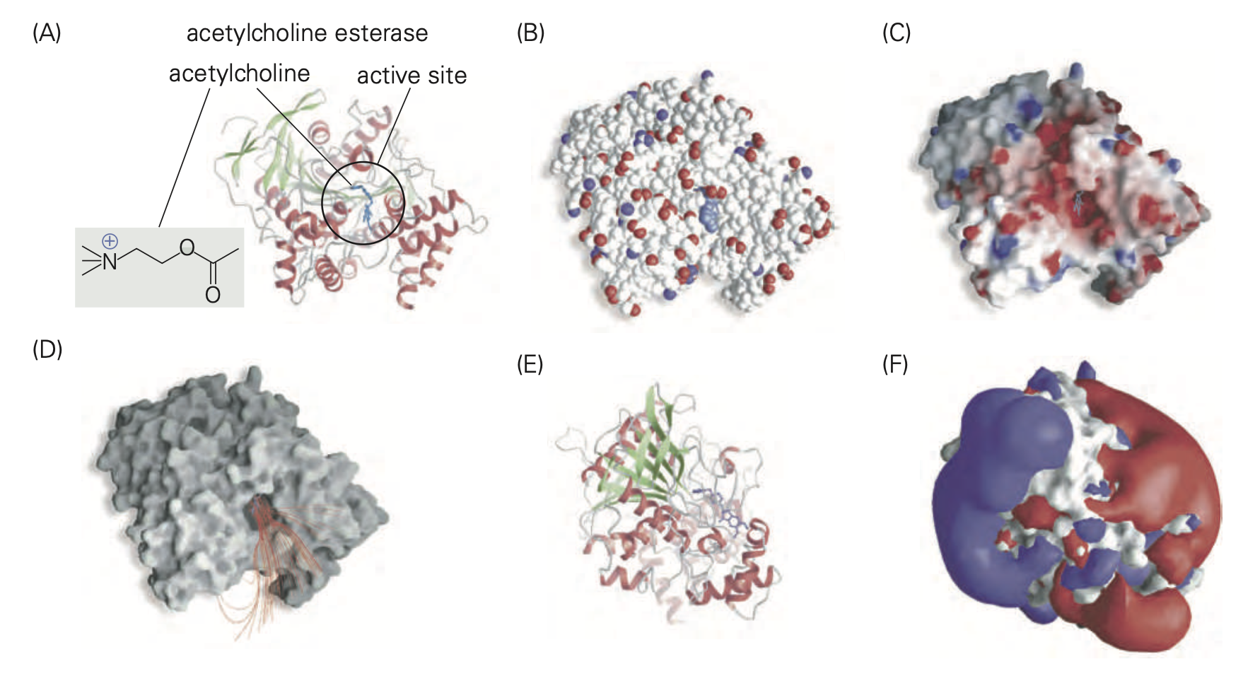
Ions screen charges. Mobile ions arrange themselves around charges so that their electric fields are reduced.
Generalized Born
 $$
U = -\frac{1}{2} \sum_{ij} \frac{q_i q_j}{f_{GB}(r_{ij}, R_i, R_j)} \left(1 - \frac{\exp[-\kappa f_{GB}]}{\varepsilon} \right)$$
where $$f_{GB} = \left[ r_{ij}^2 + R_i R_j \exp\left( -\frac{r_{ij}^2}{4 R_i R_j} \right) \right]^{1/2}$$
and $R_i$ are the effective Born radii. The effective Born radius of an atom reflects the degree of its burial inside the molecule: for an isolated ion, it is equal to its van der Waals radius. The effective radii depend on the molecule’s conformation and have to be re-computed every time the conformation changes.
The electrostatic screening effects of (monovalent) salt are incorporated via the Debye-Huckel screening parameter κ.
Poisson-Boltzmann
$$-\nabla\cdot\left[\epsilon_0\epsilon_r(\mathbf r)\nabla\psi(\mathbf r)\right] =\rho_{\rm fixed}(\mathbf r)+\sum_s q_s c_s(\mathbf r),$$
$$c_s(\mathbf r)=\chi_s(\mathbf r)c_s^{\rm bulk} \exp\!\left[-\frac{q_s\psi(\mathbf r)}{k_BT}\right].$$
- $\rho_{\rm fixed}$: solute atomic charge density.
- $\epsilon_r(\mathbf r)$: relative dielectric, different inside and outside the molecule.
- $c_s^{\rm bulk}$: bulk number density of ion species $s$; $q_s$ is its charge.
- $\chi_s$: ion accessibility, zero in the ion-excluded solute region.
Poisson relates the potential to all charges. Boltzmann describes how mobile ions redistribute in that potential.
Solve the coupled problem numerically using the molecular boundary and boundary conditions.
Beyond electrostatics
A complete implicit-solvent model also needs nonpolar solvation:
$$G_{\rm solv}\approx G_{\rm polar}^{\rm PB/GB}+G_{\rm nonpolar}.$$
A common approximation uses solvent-accessible surface area:
$$G_{\rm nonpolar}\approx aA_{\rm SASA}+b.$$
- Approximates cavity formation and solute–water interactions.
One trajectory or three?
Common workflow: explicit-solvent MD → snapshots → remove bulk solvent → endpoint evaluation.

MD–MM/PBSA for fragment selection

PurE: 352 fragments; validation by NMR and SPR.
| ROC area | MM/PBSA | GOLD docking |
|---|---|---|
| Full library (A) | 0.70 | 0.55 |
| Competition-tested subset (B) | 0.79 | 0.66 |
Reproduced from Zhu et al. · JCIM (2013), Fig. 4 and Table 1.

Ranking compounds for synthesis
16 targets, 423 binders. Relative alchemical workflows generally ranked better; performance varied by target.
Selecting the strongest of three: FEP+ 70%, MM/GBSA 49%, random 33% (target averages, Table 2).
Reproduced from Breznik et al. · ChemMedChem (2023), Fig. 4 · CC BY 4.0. MM/GBSA here uses Prime rescoring of docked poses; FEP+/PMX results were imported from literature.

Ranking and energy accuracy differ
In this benchmark, absolute FEP gave higher ranking correlations and lower offset-corrected errors.
ocRMSE removes a fitted mean error for each target; even corrected MM/GBSA errors remain much larger.
MM/GBSA cost about 75× less in this configured absolute-FEP comparison.
Reproduced from Martínez León, Andersen & Hub · BindFlow · JCTC (2026), Fig. 7 · CC BY 4.0. MM/GBSA omits the separate entropy term; exclusions and cost context are in the annotation.
Key Takeaways
ANM/GNM
- Single structure $\rightarrow$ intrinsic flexibility
Coarse grained modeling
- Fewer things to simulate - less accurate but faster
- Popular for large membrane proteins, viral capsids
Implicit solvent
- shielding (water) vs screening (ions)
- Generalized Born - effective Born radii for dynamically scaling dielectric
- Poisson–Boltzmann - solves differential equation; accounts for screening (ions) and shielding
MM/PBSA and MM/GBSA
- between docking and FEP in accuracy and speed