PART 1 DUE: 11:59 PM FRIDAY, OCTOBER 2
PART 2&3 DUE: 11:59 PM THURSDAY, OCTOBER 8
In this assignment you will write two scripts, md-simulate.py and md-analyze.py, as well as answer questions about your simulation and analysis. Because your scripts will be computationally intensive, we've split the assignment into multiple parts.
Part 1
In this part you will write a general-purpose script (md-simulate.py) for taking a PDB file and simulating it with OpenMM. We will fix any issues with the structure, energy minimize the protein, solvate and neutralize the system, minimize the full system, implement a multi-step equilibration set, and then run the production simulation.
This part of the assignment is due October 2 (although late turn-ins will be accepted with minimal penalty until October 5).
First, some biology...
Ras proteins are small G proteins (they bind GTP and GDP) that are important in several cell signaling pathways, most canonically the MAPK pathway, which regulates cell proliferation. Unsurprisingly, members of this pathway are often implicated as oncogenes, and Ras is no exception.
The wild-type* NRAS protein in the inactive state (GDP bound) is shown below with key motifs highlighted.
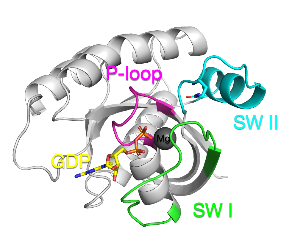
The two switch motifs (SW1 and SW2) demonstrate the largest conformational change between the GTP-bound "on" state (which triggers downstream signaling) and the GDP-bound "off" state. The P-loop binds to phosphate in GDP/GTP.
We will investigate the Q61R mutation of the NRAS protein. This mutation (or the similar Q61K) is present in 20% of cutaneous melanomas (skin cancer) and correlates with more aggressive disease progression. In this assignment we will investigate the effect of this mutation on the intrinsic dynamics of NRAS. In later assignments we will investigate its effect on ligand and protein binding.
Preparing the Q61R Structure
Your first task is to extract only the chain A protein from PDB 6ZIO, removing water, ions, GDP, and the other chain, and use the PyMOL mutagenesis wizard to mutate glutamine 61 to arginine.
The wizard will suggest what it thinks is the best rotamer for arginine based on minimizing clashes, but you should inspect the other options (flip through the available frames) to see if there is a side-chain rotamer that you like better (e.g., one that has minimal clashes but pre-forms an interaction).
Make sure you have mutated the correct residue.
Implementing md-simulate.py
Your next task is to implement the missing sections of the following script:
Follow the instructions in the comments of the script. If a setting is not specified, use the default.
Use:
- the AMBER14 force field
- TIP3P water
- the LangevinMiddleIntegrator
- a 2 fs timestep
Once your script is working (as verified by the autograder), produce 250 ns of simulation of your Q61R mutant.
Do not procrastinate running your production simulation once you have a working script. The simulation may take days to complete, and you should leave time to both perform the analysis and potentially re-run the simulation if you realize there was an error.
Inspecting Your Trajectory
You should look at the trajectories you are generating. You can use PyMOL:
pymol system.pdb etrajectory.dcd
If this is using too much memory, you can adjust the trajectory import options by deferring builds and/or downsampling the trajectory by increasing the interval.
VMD is also an option for viewing trajectories efficiently.
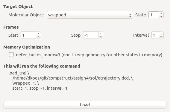
When you look at your trajectory you should immediately notice something odd: the protein appears to jump to the corner of the water box.
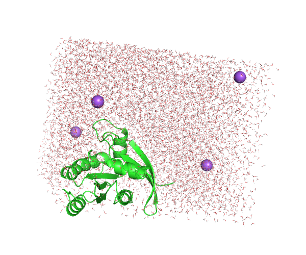
This is not a bug!
Recall that we are, in theory, simulating an infinite number of repeating periodic boxes. OpenMM, for whatever reason, likes to place the protein at the origin of the periodic box. Atoms of the same molecule are not wrapped onto the other side of the periodic box, but if you look carefully you can see the hole in the water where the protein is intruding into the other side of the box.
If this isn't making sense, please ask a question in office hours or class.
For this assignment we aren't explicitly looking at interactions with water, so we aren't going to worry too much about where the water is. However, if it bothers you, here is a script for wrapping the water into a box with the protein at the center:
Using the GPU Cluster
You should do all your evaluation of your script on a machine with a good GPU, which will be more than 100 times faster than running on only a CPU.
This means you need to figure out how to use the cluster if you haven't already.
First, work in an interactive session. Then submit the full 250 ns production simulation using sbatch.
If you don't use a GPU, you literally will be unable to finish the assignment before the due date because your simulation will still be running.
The provided script includes a reporter that will print out the speed of the simulation in nanoseconds per day. If this isn't in the hundreds, you are doing something wrong.
Grading
The autograder will attempt to check that your equilibration trajectory is doing the right thing and run a few steps of the production simulation.
Because the autograder doesn't have a GPU, this will take long enough as it is. In fact, I would have much preferred a longer equilibration time, but that simply took too long.
Do your best to validate that your script is doing what it is supposed to do by inspecting the state reported in the CSV files before submitting to the autograder.
It should only take you a minute or two to equilibrate on a GPU, but it will take the autograder about half an hour.
IMPORTANT: Due to time limitations on the autograder, we aren't equilibrating as long as we should. This means there is a chance, if you get a bad random seed, that your simulation will "blow up" and generate NaNs. If this happens with the autograder, but doesn't happen when you run the code yourself, just resubmit.
Once you have passed the autograder for this step, submit a full 250 ns simulation and start working on the next part.
Cluster Usage
Recall that to get an interactive job with a GPU on the cluster you will run:
srun --pty -p dept_gpu --gres=gpu:1 /bin/bash
This is useful for debugging and setting up your system.
Since your production simulation will take days to run, it should be submitted as a batch (non-interactive) job.
It is important that you write your trajectory to the cluster node's local hard drive (/scr) to avoid overloading the network file server that your home directory is on.
Below is an example SLURM script for running your simulation as a batch job. Submit it with sbatch.
#!/bin/bash
#SBATCH --job nras
#SBATCH --nodes=1
#SBATCH --partition=dept_gpu
#SBATCH --gres=gpu:1

# Scratch drive folder to work in
SCRDIR=/scr/${SLURM_JOB_ID}
mkdir -p $SCRDIR
chmod +rX $SCRDIR
echo scratch drive ${SCRDIR}

cp $SLURM_SUBMIT_DIR/*.pdb ${SCRDIR}
cd ${SCRDIR}

# Set up to copy files back to working dir on exit
trap "mv *dcd $SLURM_SUBMIT_DIR" EXIT

# Run the MD in the conda environment "struct"
conda run -n struct md-simulate.py --pdb nras.pdb
You can use squeue to check the status of your job:
squeue -u $USER
*Actually, this structure isn't wild-type—it has the C118S mutation, which reduces tumorigenesis in mice. It removes redox-dependent activation of NRAS. For simplicity, we will leave the mutation in the structure.
Part 2
In this part of the assignment you will write md-analysis.py, which will take a topology and trajectory file and generate a number of graphs analyzing the trajectory, as well as dumping the raw data to NumPy files for autograding.
Your script will be autograded using the following wild-type topology and trajectory. The graphs on this page were generated using these files:
This trajectory has been downsampled so each frame represents 100 ps of simulation time for faster grading. The full trajectory (without water) is available here and will be useful in Part 3.
In Part 3 of the assignment, you will be asked to upload and interpret the graphs generated by analyzing your simulation of the Q61R mutant from Part 1.
You do not have to match the formatting of the example graphs exactly, but all axes and series must be labeled.
Implement all the parts delineated in the starter code:
Preprocessing
We are only going to analyze the protein, so we can remove the solvent. This should let us keep the entire trajectory in memory for much faster processing. The original trajectory should be about 6.8 GB, while the trajectory without solvent should be about 0.8 GB.
Follow these instructions for how to create an in-memory trajectory of a subsystem.
RMSD
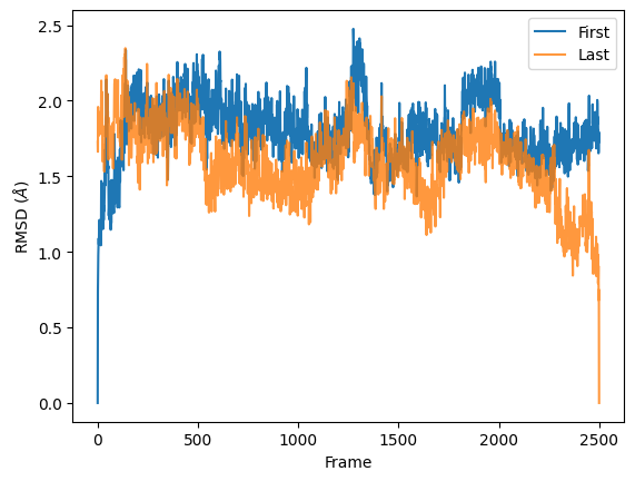
Align the trajectory to the first frame, in memory, using all the backbone atoms (not just alpha carbons).
Using this aligned trajectory, compute the RMSD of each frame relative to:
- the first frame
- the last frame
Generate the following plot. Your trajectory will not be downsampled and therefore should contain more frames.
RMSF
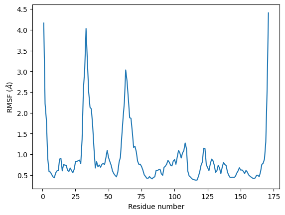
Calculate the root mean square fluctuations (RMSF) of the alpha carbons using these instructions.
Note that unlike in recitation, where we aligned to the first frame of the simulation, these instructions align to an average structure.
Even though we are only calculating RMSF for alpha carbons, so there is one number per residue, continue to align using the full backbone.
Generate the following graph:
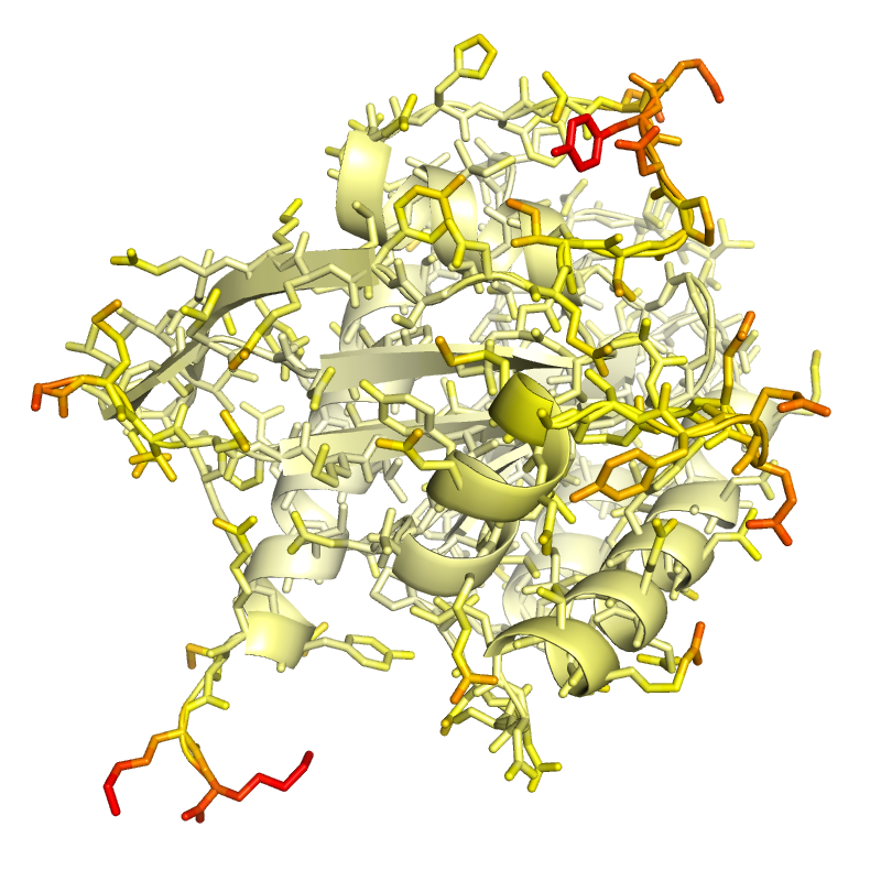
Now calculate the RMSF for all atoms and set the tempfactor of each atom equal to its RMSF, as described in the "Visualising RMSF as B-factors" section of the link above.
Write out a PDB file with these tempfactors set and visualize the structure in PyMOL.
In PyMOL:
- remove hydrogens
- use cartoon and stick representations
- color by the B-factor, which contains the RMSF values, using:
spectrum b, white_yellow_orange_red, minimum=0, maximum=6
Save a ray-traced image for uploading in the next part.
Angle Distributions
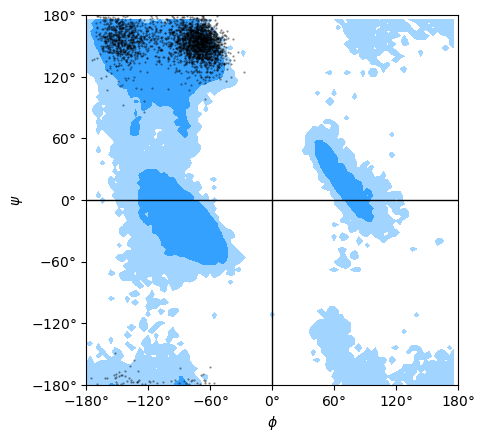
Generate a Ramachandran plot for residue 61.
Make sure you are selecting the correct residue: glutamine in wild type and arginine in the mutant.
Show the reference distribution in the background.
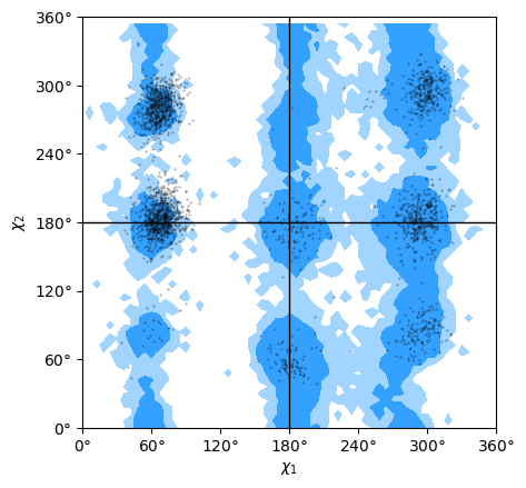
Generate a Janin plot for the same residue.
A Janin plot is similar to a Ramachandran plot, but examines the first two side-chain dihedral angles instead of the backbone dihedral angles.
Show the reference distribution in the background.
Additional Analysis
In the next part you will implement an additional analysis of your choice to characterize the difference in dynamics between wild-type and Q61R NRAS.
The goal is to identify an insightful analysis that succinctly represents these changes.
In addition to performing the analyses described above, you should spend some time looking at the simulation behavior in PyMOL.
Part 3
Answer the GradeScope questions.